Join our workshop on Cluster Analysis in R which is a part of our workshops for Ukraine series!
Here’s some more info:
Title: Cluster Analysis in R
Date: Thursday, June 6th, 18:00 – 20:00 CEST (Rome, Berlin, Paris timezone)
Speaker: Sejal Davla is a neuroscientist and data scientist who works with industry and government clients on projects at the intersection of science, data, and policy. She received her PhD in neuroscience from McGill University in Canada, where her research identified new pathways in brain development and sleep. She is an advocate for open science and reproducibility and runs R programming workshops to promote best data practices.
Description: Some datasets are unlabeled without obvious classifiers. Unsupervised machine learning methods, such as clustering, allow finding patterns and homogeneous subgroups in unlabeled data. This workshop will cover the basics of cluster analysis and how to perform clustering using k-means and hierarchical clustering methods. The goal of the workshop is to help identify datasets for clustering, learn to visualize and interpret models, validate clusters, and highlight practical issues.
Minimal registration fee: 20 euro (or 20 USD or 800 UAH)
Save your donation receipt (after the donation is processed, there is an option to enter your email address on the website to which the donation receipt is sent)
Fill in the registration form, attaching a screenshot of a donation receipt (please attach the screenshot of the donation receipt that was emailed to you rather than the page you see after donation).
If you are not personally interested in attending, you can also contribute by sponsoring a participation of a student, who will then be able to participate for free. If you choose to sponsor a student, all proceeds will also go directly to organisations working in Ukraine. You can either sponsor a particular student or you can leave it up to us so that we can allocate the sponsored place to students who have signed up for the waiting list.
Save your donation receipt (after the donation is processed, there is an option to enter your email address on the website to which the donation receipt is sent)
Fill in the sponsorship form, attaching the screenshot of the donation receipt (please attach the screenshot of the donation receipt that was emailed to you rather than the page you see after the donation). You can indicate whether you want to sponsor a particular student or we can allocate this spot ourselves to the students from the waiting list. You can also indicate whether you prefer us to prioritize students from developing countries when assigning place(s) that you sponsored.
If you are a university student and cannot afford the registration fee, you can also sign up for the waiting listhere. (Note that you are not guaranteed to participate by signing up for the waiting list).
You can also find more information about this workshop series, a schedule of our future workshops as well as a list of our past workshops which you can get the recordings & materials here.
Looking forward to seeing you during the workshop!
Hello everyone!
I’m excited to announce the release of our latest collaborative effort (R package), designed to make complex consumer price and inflation calculations a breeze: emWeightedCPI .
Here I will Introduce you to what this package is about.
What is emWeightedCPI?
Our R package “emWeightedCPI” (hosted on github) stands for Expenditure based and Multivariate Weighted Consumer Price Index. This is the result of the combined effort of myself and two other talented individuals; Dr Paul A. Agbodza and George K. Agyen . It is a versatile tool that simplifies the calculation of standard Consumer Price Indices (CPI) and Inflation using Expenditure based and Multivariate Weights. The package automates a proposed multivariate weighted indexing scheme for price data. More information can be found [here].
Why Create emWeightedCPI Package?
Normally CPI is calculated from household expenditure data obtained from household expenditure surveys. However, these surveys are expensive making it difficult to conduct on a regular basis. This package introduces an alternative weighting approach that enables the computation of variable weights using price data only.
This approach is convenient since it does not require incurring additional cost for conducting household expenditure survey to generate CPI for the determination of inflation figures. Even so, one can still generate the Laspeyres’ CPI and inflation using this package.
The workings of The package
Using emWeightedCPI is as easy as taking a stroll! Begin by installing the package from github by using
Once installed, load the package into your R environment with library(emWeightedCPI) . Now you’re all set to dive into the world emWeightedCPI and make use of its functions
How does emWeightedCPI work?
The package contains four main functions:
mvw_cpi: This function calculates the multivariate weighted indices . It requires only one argument (data); a price dataset containing prices of various items for a base year and a current year. It then calculates four index values (CPI values) based on the data provided and returns them as a named vector
mvw_inflation: Using the index values calculated by mvw_cpi, the mvw_inflation function computes the inflation rate based on the selected index. The function takes two arguments index and data . the index argument takes one of four possible values (indexes); ‘fisher’, ‘paashe’,‘laspeyres’ and ‘drobish’. The data argument requires the price dataset from which the inflation is to be determined.
eb_cpi: This function calculates consumer price indexI from expenditure based expenses. The function takes in two inputs, a price data and an expenditure data. The index calculated from this function is the ‘Laspeyres index’
eb_inflation: Like the mvw_inflation function, the eb_inflation function also calculates inflation based on the index calculated from the eb_cpi function. The function takes the same arguments specified in the eb_cpi function.
Usage Examples
Lets create a price data containing the prices of 4 different items for a base year and current year.
#create an arbitrary price data
mypriceData <- data.frame(x1=runif(50, 9.9, 13.7), x2=rnorm(50, 10.9, 2.1), x3=runif(50, 12.2, 15), x4=runif(50,19.4, 24), # base year prices y1=runif(50, 26, 30), y2=runif(50, 31, 38.9), y3=runif(50, 28.2, 33.1), y4=runif(50, 51.8, 60)# current year prices )
To calculate the multivariate weighted indices simply use;
library(emWeightedCPI)
indices <- mvw_cpi(data = mypriceData)
indices
To calculate the multivariate weighted inflation based on a specific index (let’s say ‘fishers’) we use;
inflation_value <- mvw_inflation(index = ‘fisher’, data = mypriceData) inflation_value
The expenditure based index eb_cpi and inflation eb_inflation can also be calculated easily by using the codes as shown below. We need to generate an expenditure data to use together with our previously created price data in order to calculate the expenditure based index and inflation.
#pick the average base year prices from mypriceData
n_vec <- apply(mypriceData[, 1:4], 2, mean)
n_vec
#combine the output above into a dataframe with two columns and same
#number of rows as number of price items to create expenditure data
Innovation often thrives when minds come together, and emWeightedCPI is a testament to the power of collaboration. We’re incredibly proud of what we’ve achieved with this package, and we hope it becomes a valuable asset in your analytical toolkit.
Why Use emWeightedCPI?
Ease of Use: The functions in emWeightedCPI are designed to be intuitive and straightforward to use.
Flexibility: Users can customize the calculations based on their specific requirements by adjusting the input parameters especially for the mvw_inflation function
Efficiency: With optimized algorithms, emWeightedCPI delivers fast and accurate results.
Get Started with emWeightedCPI Today!
If you’re looking to simplify your consumer price index and inflation rate calculations in R, give emWeightedCPI a try! You can install it directly from github using:
Join our workshop on Conducting Simulation Studies in R, which is a part of our workshops for Ukraine series!
Here’s some more info:
Title: Conducting Simulation Studies in R
Date: Thursday, May 23rd, 18:00 – 20:00 CEST (Rome, Berlin, Paris timezone)
Speaker: Greg Faletto is a statistician and data scientist at VideoAmp, where he works on causal inference. Greg completed his Ph.D. in statistics at the University of Southern California in 2023. His research focused on developing machine learning methods has been published in venues like the International Conference on Machine Learning and the Proceedings of the National Academy of Sciences. Greg has taught classes at USC on data science and communicating insights from data, and he has previously presented his research and led workshops at venues including USC, the University of California San Francisco, the University of Copenhagen, Data Con LA, and IM Data Conference.
Description: In simulation studies (also known as Monte Carlo simulations or synthetic data experiments), we generate data sets according to a prespecified model, perform some calculations on each data set, and analyze the results. Simulation studies are useful for testing whether a methodology will work in a given setting, assessing whether a model “works” and diagnosing problems, evaluating theoretical claims, and more. In this workshop, I’ll walk through how you can use the R simulator package to conduct simple, reproducible simulation studies. You’ll learn how to carry out the full process, including making plots or tables of your results.
Minimal registration fee: 20 euro (or 20 USD or 800 UAH)
Save your donation receipt (after the donation is processed, there is an option to enter your email address on the website to which the donation receipt is sent)
Fill in the registration form, attaching a screenshot of a donation receipt (please attach the screenshot of the donation receipt that was emailed to you rather than the page you see after donation).
If you are not personally interested in attending, you can also contribute by sponsoring a participation of a student, who will then be able to participate for free. If you choose to sponsor a student, all proceeds will also go directly to organisations working in Ukraine. You can either sponsor a particular student or you can leave it up to us so that we can allocate the sponsored place to students who have signed up for the waiting list.
Save your donation receipt (after the donation is processed, there is an option to enter your email address on the website to which the donation receipt is sent)
Fill in the sponsorship form, attaching the screenshot of the donation receipt (please attach the screenshot of the donation receipt that was emailed to you rather than the page you see after the donation). You can indicate whether you want to sponsor a particular student or we can allocate this spot ourselves to the students from the waiting list. You can also indicate whether you prefer us to prioritize students from developing countries when assigning place(s) that you sponsored.
If you are a university student and cannot afford the registration fee, you can also sign up for the waiting listhere. (Note that you are not guaranteed to participate by signing up for the waiting list).
You can also find more information about this workshop series, a schedule of our future workshops as well as a list of our past workshops which you can get the recordings & materials here.
Looking forward to seeing you during the workshop!
Join our workshop on Optimal policy learning based on causal machine learning in R, which is a part of our workshops for Ukraine series!
Here’s some more info:
Title: Optimal policy learning based on causal machine learning in R
Date: Thursday, May 16th, 18:00 – 20:00 CEST (Rome, Berlin, Paris timezone)
Speaker: Martin Huber earned his Ph.D. in Economics and Finance with a specialization in econometrics from the University of St. Gallen in 2010. Following this, he served as an Assistant Professor of Quantitative Methods in Economics at the same institution. He undertook a visiting appointment at Harvard University in 2011–2012 before joining the University of Fribourg as a Professor of Applied Econometrics in 2014. His research encompasses methodological and applied contributions across various fields, including causal analysis and policy evaluation, machine learning, statistics, econometrics, and empirical economics. Martin Huber’s work has been published in academic journals such as the Journal of the American Statistical Association, the Journal of the Royal Statistical Society B, the Journal of Econometrics, the Review of Economics and Statistics, the Journal of Business and Economic Statistics, and the Econometrics Journal, among others. He is also the author of the book “Causal Analysis: Impact Evaluation and Causal Machine Learning with Applications in R.”
Description: Causal analysis aims to assess the causal effect of a treatment, such as a training program for jobseekers, on an outcome of interest, such as employment. This assessment requires ensuring comparability between groups receiving and not receiving the treatment in terms of outcome-relevant background characteristics (e.g., education or experience). Causal machine learning serves two primary purposes: (1) generating comparable groups in a data-driven manner by detecting and controlling for characteristics that significantly affect the treatment and outcome, and (2) assessing the heterogeneity of treatment effects across groups differing in observed characteristics. Closely related to effect heterogeneity analysis is optimal policy learning, which seeks to optimally target specific subgroups with treatment based on their observed characteristics to maximize treatment effectiveness. This workshop introduces optimal policy learning based on causal machine learning, facilitating (1) data-driven segmentation of a sample into subgroups and (2) optimal treatment assignment across subgroups to maximize effectiveness. The workshop also explores applications of this method using the statistical software “R” and its interface “R Studio.”
Minimal registration fee: 20 euro (or 20 USD or 800 UAH)
Save your donation receipt (after the donation is processed, there is an option to enter your email address on the website to which the donation receipt is sent)
Fill in the registration form, attaching a screenshot of a donation receipt (please attach the screenshot of the donation receipt that was emailed to you rather than the page you see after donation).
If you are not personally interested in attending, you can also contribute by sponsoring a participation of a student, who will then be able to participate for free. If you choose to sponsor a student, all proceeds will also go directly to organisations working in Ukraine. You can either sponsor a particular student or you can leave it up to us so that we can allocate the sponsored place to students who have signed up for the waiting list.
Save your donation receipt (after the donation is processed, there is an option to enter your email address on the website to which the donation receipt is sent)
Fill in the sponsorship form, attaching the screenshot of the donation receipt (please attach the screenshot of the donation receipt that was emailed to you rather than the page you see after the donation). You can indicate whether you want to sponsor a particular student or we can allocate this spot ourselves to the students from the waiting list. You can also indicate whether you prefer us to prioritize students from developing countries when assigning place(s) that you sponsored.
If you are a university student and cannot afford the registration fee, you can also sign up for the waiting listhere. (Note that you are not guaranteed to participate by signing up for the waiting list).
You can also find more information about this workshop series, a schedule of our future workshops as well as a list of our past workshops which you can get the recordings & materials here.
Looking forward to seeing you during the workshop!
Join our workshop on AI Use Cases for R Enthusiasts, which is a part of our workshops for Ukraine series!
Here’s some more info:
Title: AI Use Cases for R Enthusiasts
Date: Thursday, May 9th, 18:00 – 20:00 CEST (Rome, Berlin, Paris timezone)
Speaker: Dr. Albert Rapp is a mathematician with a fascination for the blend of Data Analytics, Web Development, and Visualization. He applies his expertise as a business analyst, focusing on AI, cloud computing, and data analysis. Outside of his professional pursuits, Albert enjoys engaging with the community by sharing his insights and knowledge on platforms like LinkedIn, YouTube, and through his video courses.
Description: Everyone is talking about AI. And for good reasons: It’s a powerful tool that can enhance your productivity as a programmer as well as help you with automated data processing tasks. In this workshop, I share R-specific and general AI tools and workflows that I use for my programming, blogging and video projects. By the end of this session, participants will be equipped with fresh ideas and practical strategies for using AI in their own endeavors.
Minimal registration fee: 20 euro (or 20 USD or 800 UAH)
Save your donation receipt (after the donation is processed, there is an option to enter your email address on the website to which the donation receipt is sent)
Fill in the registration form, attaching a screenshot of a donation receipt (please attach the screenshot of the donation receipt that was emailed to you rather than the page you see after donation).
If you are not personally interested in attending, you can also contribute by sponsoring a participation of a student, who will then be able to participate for free. If you choose to sponsor a student, all proceeds will also go directly to organisations working in Ukraine. You can either sponsor a particular student or you can leave it up to us so that we can allocate the sponsored place to students who have signed up for the waiting list.
Save your donation receipt (after the donation is processed, there is an option to enter your email address on the website to which the donation receipt is sent)
Fill in the sponsorship form, attaching the screenshot of the donation receipt (please attach the screenshot of the donation receipt that was emailed to you rather than the page you see after the donation). You can indicate whether you want to sponsor a particular student or we can allocate this spot ourselves to the students from the waiting list. You can also indicate whether you prefer us to prioritize students from developing countries when assigning place(s) that you sponsored.
If you are a university student and cannot afford the registration fee, you can also sign up for the waiting listhere. (Note that you are not guaranteed to participate by signing up for the waiting list).
You can also find more information about this workshop series, a schedule of our future workshops as well as a list of our past workshops which you can get the recordings & materials here.
Looking forward to seeing you during the workshop!
After some years as a Stata user, I found myself in a new position where the tools available were SQL and SPSS. I was impressed by the power of SQL, but I was unhappy with going back to SPSS after five years with Stata.
Luckily, I got the go-ahead from my leaders at the department to start testing out R as a tool to supplement SQL in data handling.
This was in the beginning of 2020, and by March we were having a social gathering at our workplace. A Bingo night! Which turned out to be the last social event before the pandemic lockdown.
What better opportunity to learn a new programming language than to program some bingo cards! I learnt a lot from this little project.
It uses the packages grid and gridExtra to prepare and embellish the cards.
The function BingoCard draws the cards and is called from the function Bingo3. When Bingo3 is called it runs BingoCard the number of times necessary to create the requested number of sheets and stores the result as a pdf inside a folder defined at the beginning of the script.
All steps could have been added together in a single function. For instance, a more complete function could have included input for the color scheme of the cards, the number of cards on each sheet and more advanced features for where to store the results.
Still, this worked quite well, and was an excellent way of learning since it was both so much fun and gave me the opportunity to talk enthusiastically about R during Bingo Night.
library(gridExtra)
library(grid)
##################################################################
# Be sure to have a folder where results are stored
##################################################################
CardFolder <- "BingoCards"
if (!dir.exists(CardFolder)) {dir.create(CardFolder)}
##################################################################
# Create a theme to use for the cards
##################################################################
thema <- ttheme_minimal(
base_size = 24, padding = unit(c(6, 6), "mm"),
core=list(bg_params = list(fill = rainbow(5),
alpha = 0.5,
col="black"),
fg_params=list(fontface="plain",col="darkblue")),
colhead=list(fg_params=list(col="darkblue")),
rowhead=list(fg_params=list(col="white")))
##################################################################
## Define the function BingoCard
##################################################################
BingoCard <- function() {
B <- sample(1:15, 5, replace=FALSE)
I <- sample(16:30, 5, replace=FALSE)
N <- sample(31:45, 5, replace=FALSE)
G <- sample(46:60, 5, replace=FALSE)
O <- sample(61:75, 5, replace=FALSE)
BingoCard <- as.data.frame(cbind(B,I,N,G,O))
BingoCard[3,"N"]<-"X"
a <- tableGrob(BingoCard, theme = thema)
return(a)
}
##################################################################
## Define the function Bingo3
## The function has two arguments
## By default, 1 sheet with 3 cards is stored in the CardFolder
## The default name is "bingocards.pdf"
## This function calls the BingoCard function
##################################################################
Bingo3 <- function(NumberOfSheets=1, SaveFileName="bingocards") {
myplots <- list()
N <- NumberOfSheets*3
for (i in 1 : N ) {
a1 <- BingoCard()
myplots[[i]] <- a1
}
ml <- marrangeGrob(myplots, nrow=3, ncol=1,top="")
save_here <- paste0(CardFolder,"/",SaveFileName,".pdf")
ggplot2::ggsave(save_here, ml, device = "pdf", width = 210,
height = 297, units = "mm")
}
##################################################################
## Run Bingo3 with default values
##################################################################
Bingo3()
##################################################################
## Run Bingo3 with custom values
##################################################################
Bingo3(NumberOfSheets = 30, SaveFileName = "30_BingoCards")
In previous article, I introduced method to share shiny application in static web page (github page)
At the core of this method is a technology called WASM, which is a way to load and utilize R and Shiny-related libraries and files that have been converted for use in a web browser. The main problem with wasm is that it is difficult to configure, even for R developers.
Of course, there was a way called shinylive, but unfortunately it was only available in python at the time.
Fortunately, after a few months, there is an R package that solves this configuration problem, and I will introduce how to use it to add a shiny application to a static page.
shinylive
shinylive is R package to utilize wasm above shiny. and now it has both Python and R version, and in this article will be based on the R version.
shinylive is responsible for generating HTML, Javascript, CSS, and other elements needed to create web pages, as well as wasm-related files for using shiny.
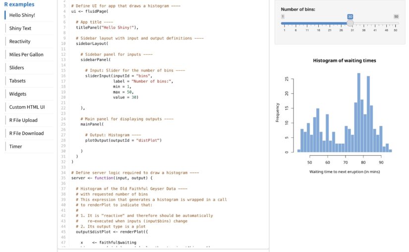
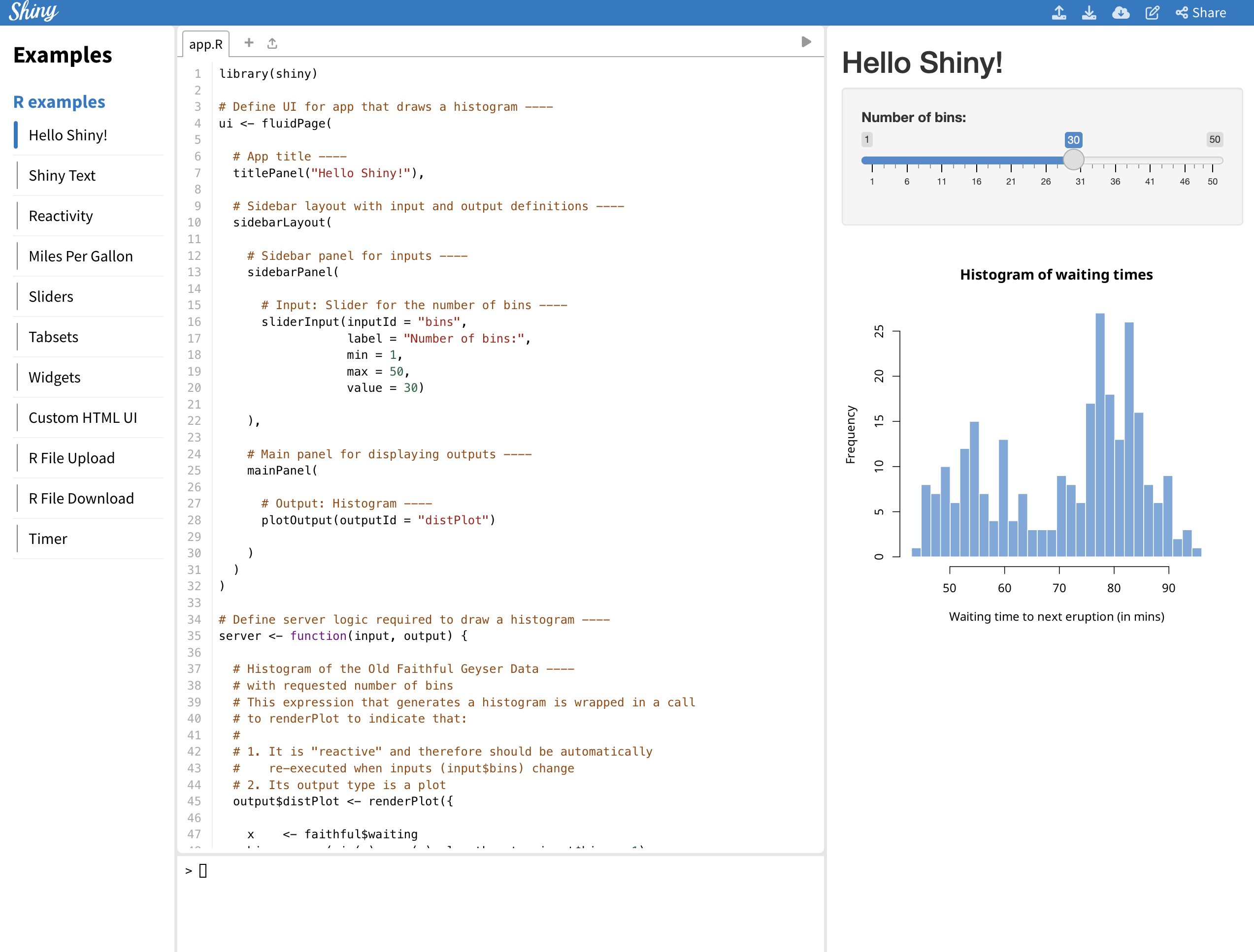
You can see examples created with shinylive at this link.
Install shinylive
While shinylive is available on CRAN, it is recommended to use the latest version from github as it may be updated from time to time, with the most recent release being 0.1.1. Additionally, pak is the recently recommended R package for installing R packages in posit, and can replace existing functions like install.packages() and remotes::install_github().
You can think of shinylive as adding a wasm to an existing shiny application, which means you need to create a shiny application first.
For the example, we’ll use the code provided by shiny package (which you can also see by typing shiny::runExample("01_hello") in the Rstudio console).
library(shiny)

ui <- fluidPage(

titlePanel("Hello Shiny!"),
  sidebarLayout(
  sidebarPanel(
    sliderInput(
      inputId = "bins",
      label = "Number of bins:",
      min = 1,
      max = 50,
      value = 30
    )
  ),
  mainPanel(
    plotOutput(outputId = "distPlot")
    )
  )
)

server <- function(input, output) {
  output$distPlot <- renderPlot({
  x <- faithful$waiting
  bins <- seq(min(x), max(x), length.out = input$bins + 1)
  hist(x,
    breaks = bins, col = "#75AADB", border = "white",
    xlab = "Waiting time to next eruption (in mins)",
    main = "Histogram of waiting times"
  )
  })
}

shinyApp(ui = ui, server = server)
This code creates a simple shiny application that creates a number of histograms in response to the user’s input, as shown below.
There are two ways to create a static page with this code using shinylive, one is to create it as a separate webpage (like previous article) and the other is to embed it as internal content on a quarto blog page .
First, here’s how to create a separate webpage.
shinylive via web page
To serve shiny on a separate static webpage, you’ll need to convert your app.R to a webpage using the shinylive package you installed earlier.
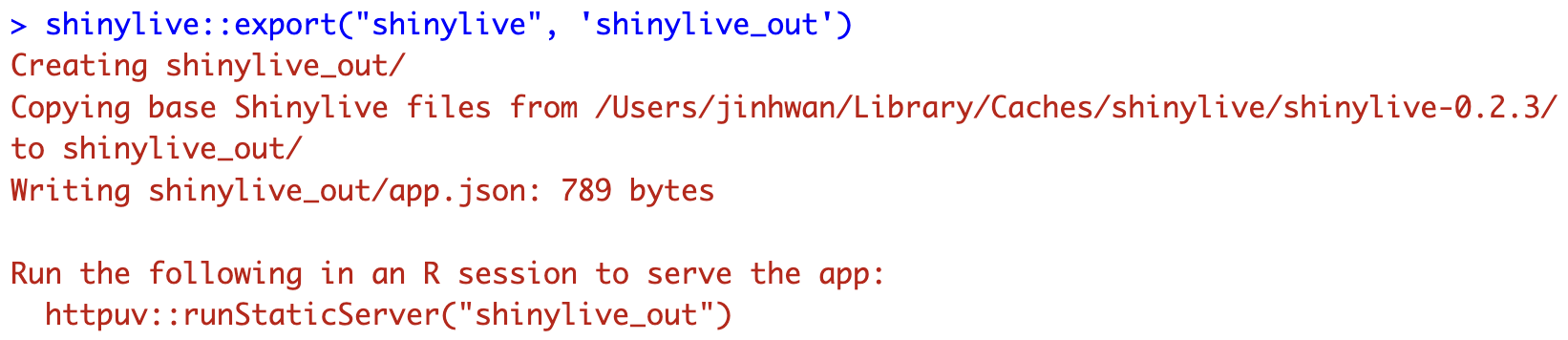
Based on creating a folder named shinylive in my Documents(~/Documents) and saving `app.R` inside it, here’s an example of how the export function would look like shinylive::export('~/Documents/shinylive', '~/Documents/shinylive_out')
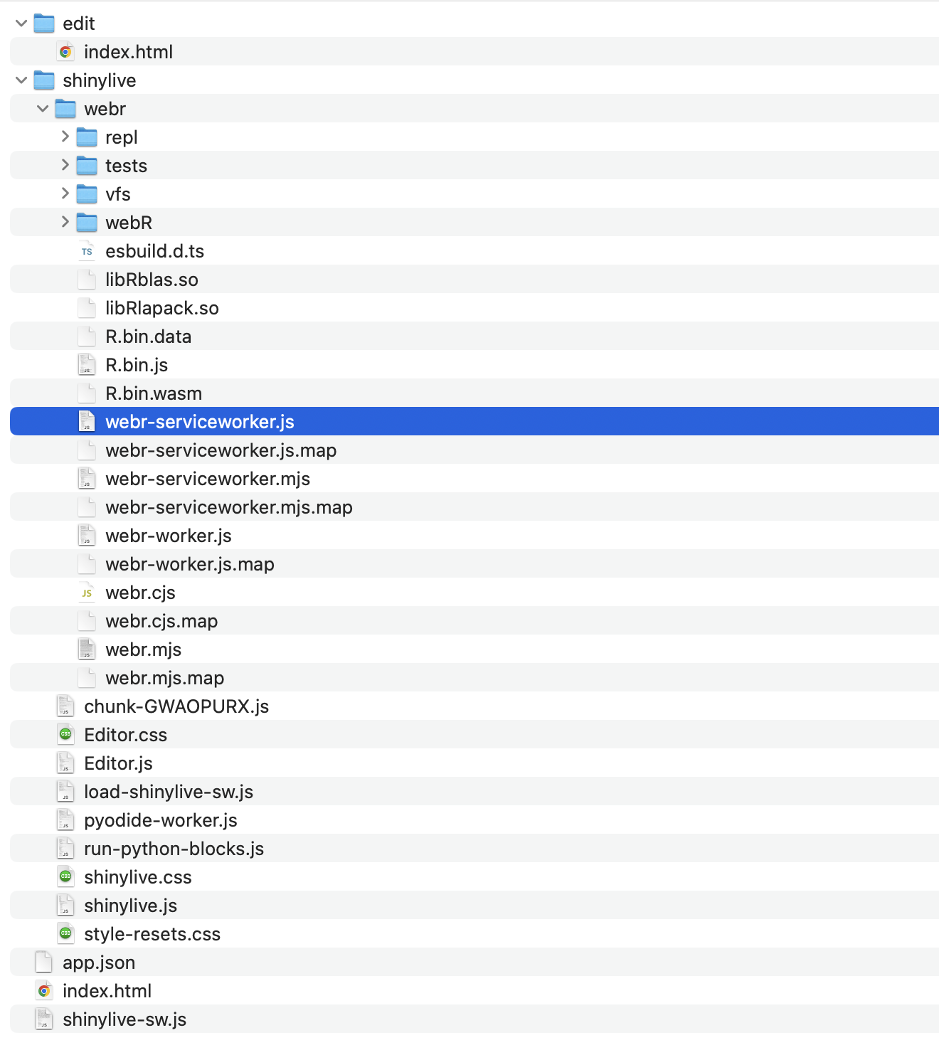
When you run this code, it will create a new folder called shinylive_out in the same location as shinylive, (i.e. in My Documents), and inside it, it will generate the converted wasm version of shiny code using the shinylive package.
If you check the contents of this shinylive_out folder, you can see that it contains the webr, service worker, etc. mentioned in the previous post.
More specifically, the export function is responsible for adding the files from the local PC’s shinylive package assets, i.e. the library files related to shiny, to the out directory on the local PC currently running R studio.
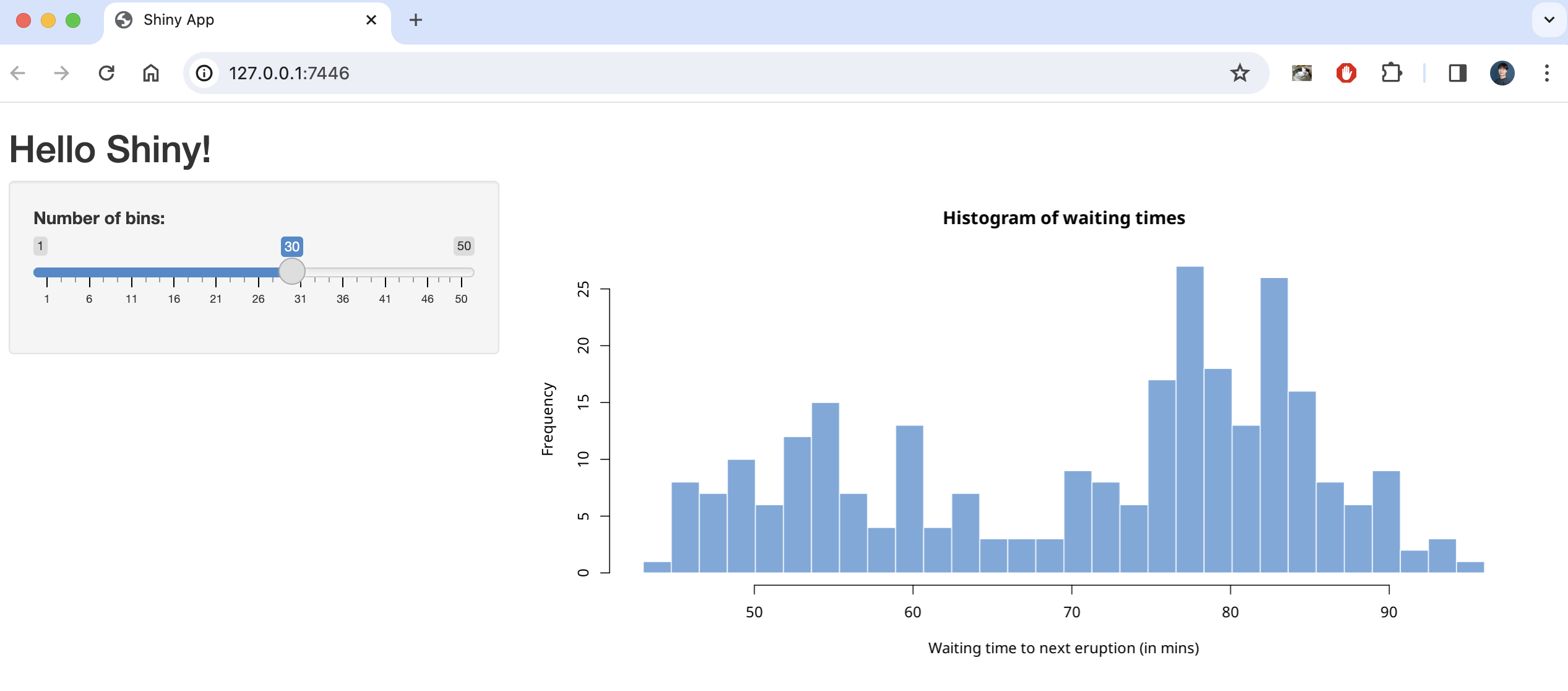
Now, if you create a github page or something based on the contents of this folder, you can serve a static webpage that provides shiny, and you can preview the result with the command below.
To add a shiny application to a quarto blog, you need to use a separate extension. The quarto extension is a separate package that extends the functionality of quarto, similar to using R packages to add functionality to basic R.
First, we need to add the quarto extension by running the following code in the terminal (not a console) of Rstudio.
quarto add quarto-ext/shinylive
You don’t need to create a separate file to plant shiny in your quarto blog, you can use a code block called {shinylive-r}. Additionally, you need to set shinylive in the yaml of your index.qmd.
filters:
- shinylive
Then, in the {shinylive-r} block, write the contents of the app.R we created earlier.
#| standalone: true
#| viewerHeight: 800
library(shiny)
ui <- fluidPage(
  titlePanel("Hello Shiny!"),
  sidebarLayout(
    sidebarPanel(
      sliderInput(
        inputId = "bins",
        label = "Number of bins:",
        min = 1,
        max = 50,
        value = 30
      )
    ),
    mainPanel(
      plotOutput(outputId = "distPlot")
    )
  )
)
server <- function(input, output) {
  output$distPlot <- renderPlot({
    x <- faithful$waiting
    bins <- seq(min(x), max(x), length.out = input$bins + 1)
    hist(x,
      breaks = bins, col = "#75AADB", border = "white",
      xlab = "Waiting time to next eruption (in mins)",
      main = "Histogram of waiting times"
    )
  })
}
shinyApp(ui = ui, server = server)
after add this in quarto blog, you may see working shiny application.
shinylive is a feature that utilizes wasm to run shiny on static pages, such as GitHub pages or quarto blogs, and is available as an R package and quarto extension, respectively.
Of course, since it is less than a year old, not all features are available, and since it uses static pages, there are disadvantages compared to utilizing a separate shiny server.
However, it is very popular for introducing shiny usage and simple statistical analysis, and you can practice it right on the website without installing R, and more features are expected to be added in the future.
The code used in blog (previous example link) can be found at the link.
Join our workshop on Introduction to Causal Machine Learning estimators in R, which is a part of our workshops for Ukraine series!
Here’s some more info:
Title: Introduction to Causal Machine Learning estimators in R
Date: Thursday, April 11th, 18:00 – 20:00 CET (Rome, Berlin, Paris timezone)
Speaker: Michael Knaus is Assistant Professor of “Data Science in Economics” at the University of Tübingen. He is working at the intersection of causal inference and machine learning for policy evaluation and recommendation.
Description: You want to learn about Double Machine Learning and/or Causal Forests for causal effect estimation but are hesitant to start because of the heavy formulas involved? Or you are already using them and curious to (better) understand what happens under the hood? In this course, we take a code first, formulas second approach. You will see how to manually replicate the output of the powerful DoubleML and grf packages using at most five lines of code and nothing more than OLS. After seeing that everything boils down to simple recipes, the involved formulas will look more friendly. The course establishes therefore how things work and gives references to further understand why things work.
Minimal registration fee: 20 euro (or 20 USD or 800 UAH)
Save your donation receipt (after the donation is processed, there is an option to enter your email address on the website to which the donation receipt is sent)
Fill in the registration form, attaching a screenshot of a donation receipt (please attach the screenshot of the donation receipt that was emailed to you rather than the page you see after donation).
If you are not personally interested in attending, you can also contribute by sponsoring a participation of a student, who will then be able to participate for free. If you choose to sponsor a student, all proceeds will also go directly to organisations working in Ukraine. You can either sponsor a particular student or you can leave it up to us so that we can allocate the sponsored place to students who have signed up for the waiting list.
Save your donation receipt (after the donation is processed, there is an option to enter your email address on the website to which the donation receipt is sent)
Fill in the sponsorship form, attaching the screenshot of the donation receipt (please attach the screenshot of the donation receipt that was emailed to you rather than the page you see after the donation). You can indicate whether you want to sponsor a particular student or we can allocate this spot ourselves to the students from the waiting list. You can also indicate whether you prefer us to prioritize students from developing countries when assigning place(s) that you sponsored.
If you are a university student and cannot afford the registration fee, you can also sign up for the waiting listhere. (Note that you are not guaranteed to participate by signing up for the waiting list).
You can also find more information about this workshop series, a schedule of our future workshops as well as a list of our past workshops which you can get the recordings & materials here.
Looking forward to seeing you during the workshop!
WhatsApp is one of the most heavily used mobile instant messaging applications around the world. It is especially popular for everyday communication with friends and family and most users communicate on a daily or a weekly basis through the app. Interestingly, it is possible for WhatsApp users to extract a log file from each of their chats. This log file contains all textual communication in the chat that was not manually deleted or is not too far in the past.
This logging of digital communication is on the one hand interesting for researchers seeking to investigate interpersonal communication, social relationships, and linguistics, and can on the other hand also be interesting for individuals seeking to learn more about their own chatting behavior (or their social relationships).
The WhatsR R-package enables users to transform exported WhatsApp chat logs into a usable data frame object with one row per sent message and multiple variables of interest. In this blog post, I will demonstrate how the package can be used to process and visualize chat log files.
Installing the Package The package can either be installed via CRAN or via GitHub for the most up-to-date version. I recommend to install the GitHub version for the most recent features and bugfixes.
# from CRAN
# install.packages("WhatsR")

# from GitHub
devtools::install_github("gesiscss/WhatsR")
The package also needs to be attached before it can be used. For creating nicer plots, I recommend to also install and attach the patchwork package.
Obtaining a Chat Log You can export one of your own chat logs from your phone to your email address as explained in this tutorial. If you do this, I recommend to use the “without media” export option as this allows you to export more messages.
If you don’t want to use one of your own chat logs, you can create an artificial chat log with the same structure as a real one but with made up text using the WhatsR package!
## creating chat log for demonstration purposes

# setting seed for reproducibility
set.seed(1234)

# simulating chat log
# (and saving it automatically as a .txt file in the working directory)
create_chatlog(n_messages = 20000,
               n_chatters = 5,
               n_emoji = 5000,
               n_diff_emoji = 50,
               n_links = 999,
               n_locations = 500,
               n_smilies = 2500,
               n_diff_smilies = 10,
               n_media = 999,
               n_sdp = 300,
               startdate = "01.01.2019",
               enddate = "31.12.2023",
               language = "english",
               time_format = "24h",
               os = "android",
               path = getwd(),
               chatname = "Simulated_WhatsR_chatlog")
Parsing Chat Log File Once you have a chat log on your device, you can use the WhatsR package to import the chat log and parse it into a usable data frame structure.
data <- parse_chat("Simulated_WhatsR_chatlog.txt", verbose = TRUE)
Checking the parsed Chat Log You should now have a data frame object with one row per sent message and 19 variables with information extracted from the individual messages. For a detailed overview what each column contains and how it is computed, you can check the related open source publication for the package. We also add a tabular overview here.
## Checking the chat log
dim(data)
colnames(data)
Column Name
Description
DateTime
Timestamp for date and time the message was sent. Formatted as yyyy-mm-dd hh:mm:ss
Sender
Name of the sender of the message as saved in the contact list of the exporting phone or telephone number. Messages inserted by WhatsApp into the chat are coded with “WhatsApp System Message”
Message
Text of user-generated messages with all information contained in the exported chat log
Flat
Simplified version of the message with emojis, numbers, punctuation, and URLs removed. Better suited for some text mining or machine learning tasks
TokVec
Tokenized version of the Flat column. Instead of one text string, each cell contains a list of individual words. Better suited for some text mining or machine learning tasks
URL
A list of all URLs or domains contained in the message body
Media
A list of all media attachment filenames contained in the message body
Location
A list of all shared location URLs or indicators in the message body, or indicators for shared live locations
Emoji
A list of all emoji glyphs contained in the message body
EmojiDescriptions
A list of all emojis as textual representations contained in the message body
Smilies
A list of all smileys contained in the message body
SystemMessage
Messages that are inserted by WhatsApp into the conversation and not generated by users
TokCount
Amount of user-generated tokens per message
TimeOrder
Order of messages as per the timestamps on the exporting phone
DisplayOrder
Order of messages as they appear in the exported chat log
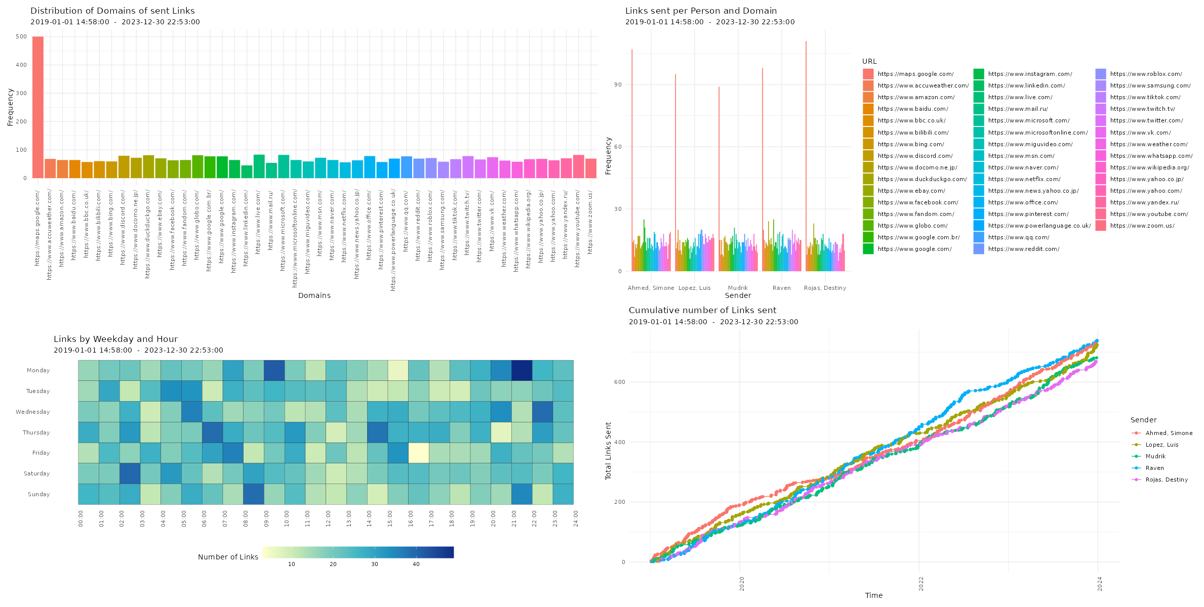
Checking Descriptives of Chat Logs Now, you can have a first look at the overall statistics of the chat log. You can check the number of messages, sent tokens, number of chat participants, date of first message, date of last message, the timespan of the chat, and the number of emoji, smilies, links, media files, as well as locations in the chat log.
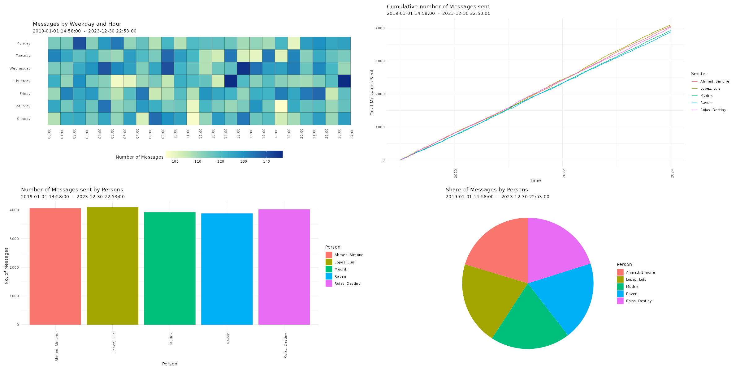
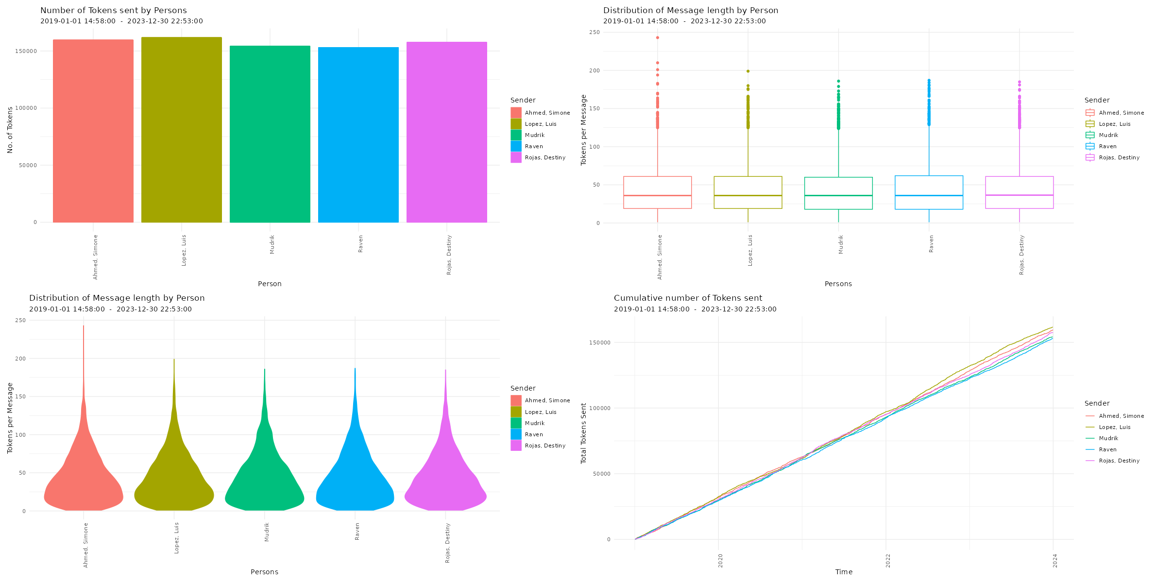
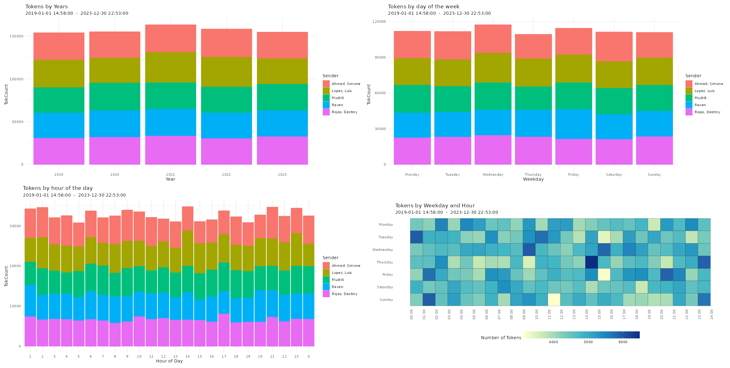
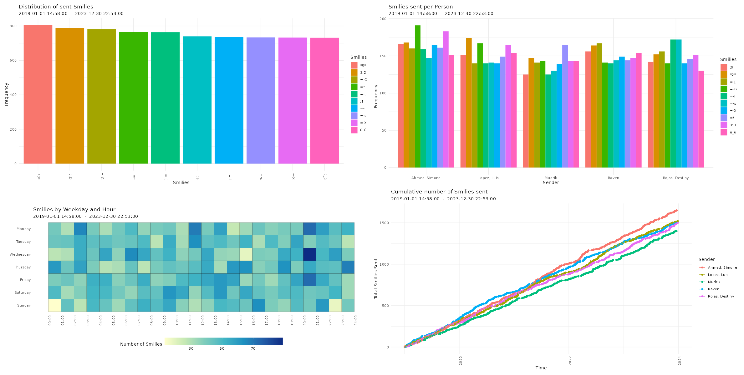
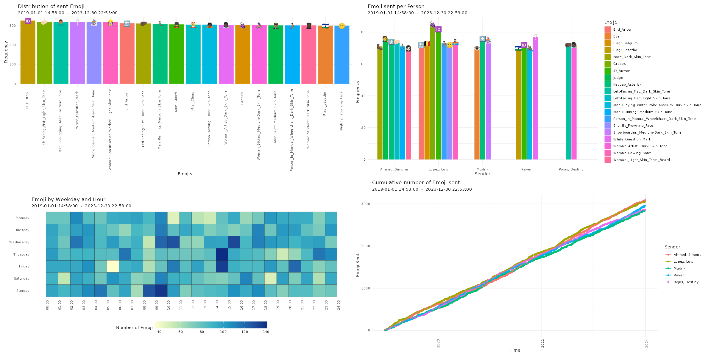
Visualizing Chat Logs The chat characteristics can now be visualized using the custom functions from the WhatsR package. These functions are basically wrappers to ggplot2 with some options for customizing the plots. Most plots have multiple ways of visualizing the data. For the visualizations, we can exclude the WhatsApp System Messages using ‘exclude_sm= TRUE’. Lets try it out:
Four different ways of visualizing the amount of sent emoji in a WhatsApp chat log. Click image to zoom in. Distribution of reaction times
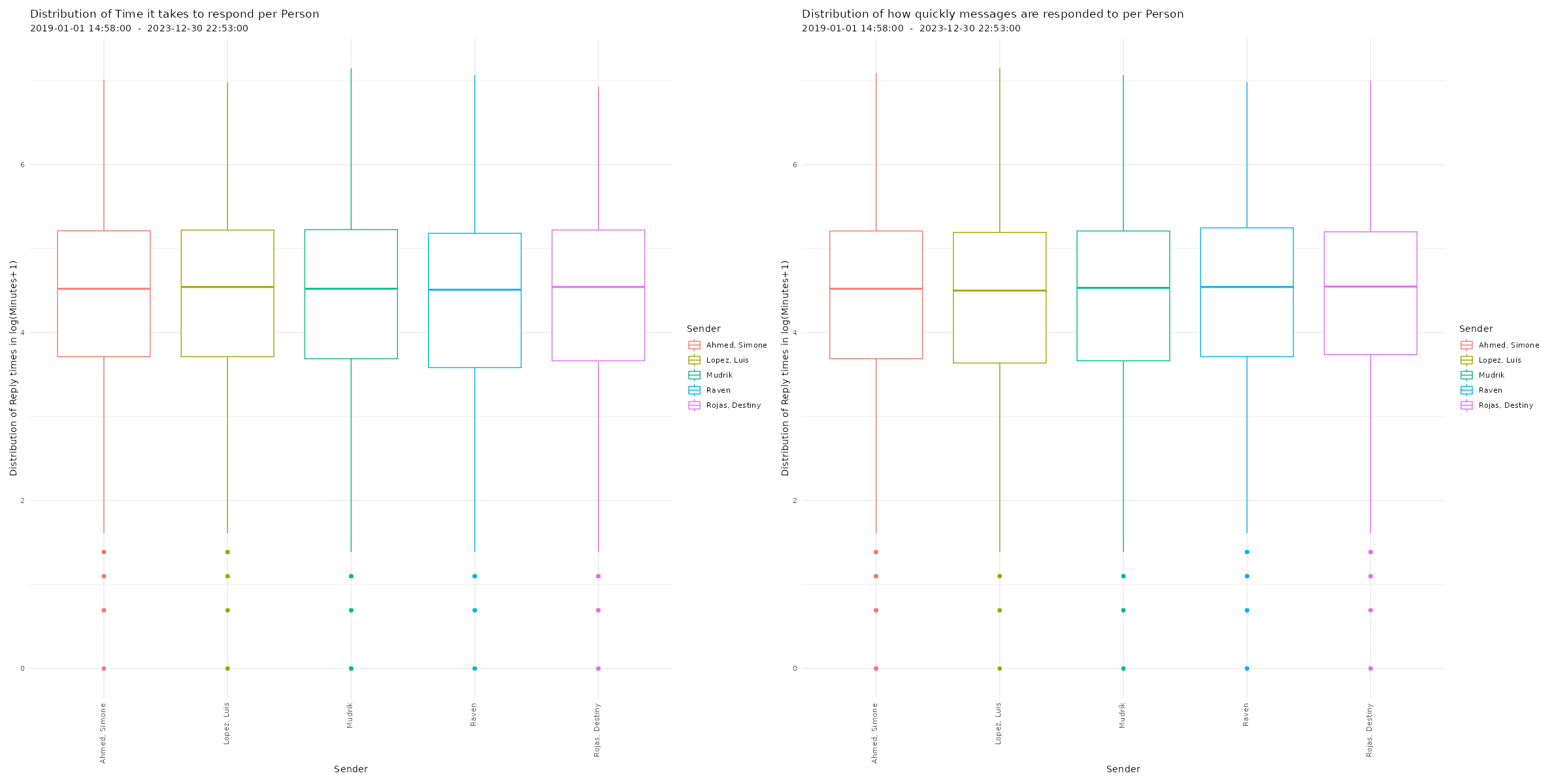
# Plotting distribution of reaction times
p26 <- plot_replytimes(data,
                       type = "replytime",
                       exclude_sm = TRUE)
p27 <- plot_replytimes(data,
                       type = "reactiontime",
                       exclude_sm = TRUE)

# Printing plots with patchwork package
free(p26) | free(p27)
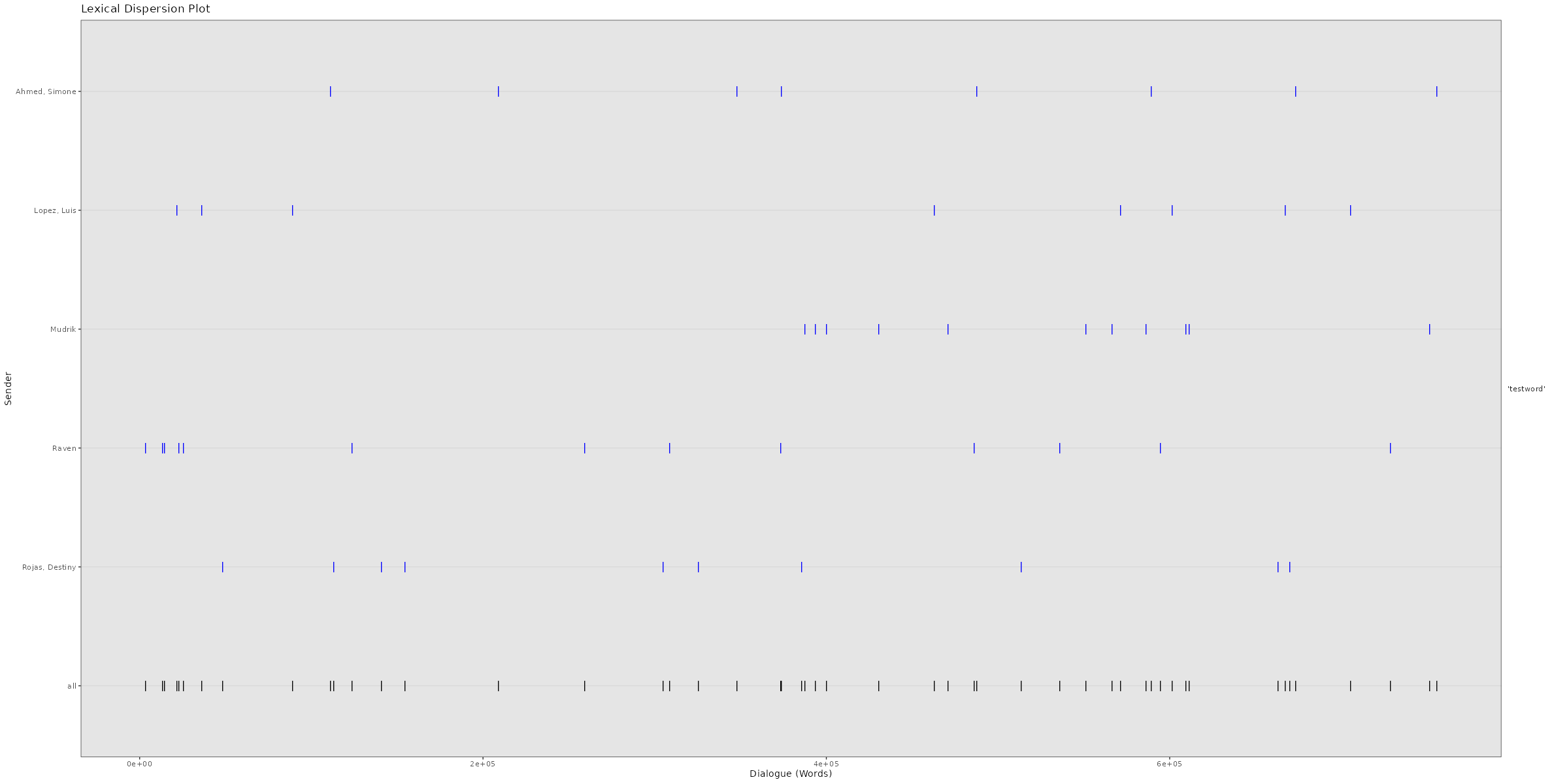
Average response times and times it takes to answer to messages for each individual chat participant in a WhatsApp chat log. Click image to zoom in. Lexical Dispersion A lexical dispersion plot is a visualization of where specific words occur within a text corpus. Because the simulated chat log in this example is using lorem ipsum text where all words occur similarly often, we add the string “testword” to a random subsample of messages. For visualizing real chat logs, this would of course not be necessary.
# Adding "testword" to random subset of messages for demonstration         # purposes
set.seed(12345)
word_additions <- sample(dim(data)[1],50)
data$TokVec[word_additions]
sapply(data$TokVec[word_additions],function(x){c(x,"testword")})
data$Flat[word_additions] <- sapply(data$Flat[word_additions],
  function(x){x <- paste(x,"testword");return(x)})
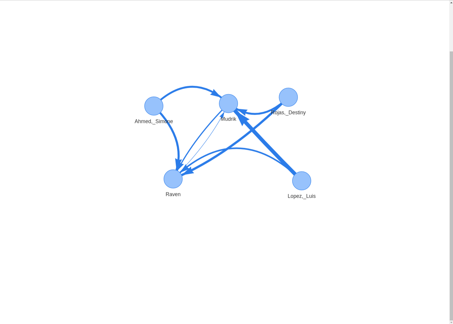
Network graph showing how often each chat participant directly responded to the previous messages (a subsequent message is counted as a “response” here). Click image to zoom in.
Issues and long-term availability.
Unfortunately, WhatsApp chat logs are a moving target when it comes to plotting and visualization. The structure of exported WhatsApp chat logs keeps changing from time to time. On top of that, the structure of chat logs is different for chats exported from different operating systems (Android & iOS) and for different time (am/pm vs. 24h format) and language (e.g. English & German) settings on the exporting phone. When the structure changes, the WhatsR package can be limited in its functionality or become completely dysfunctional until it is updated and tested. Should you encounter any issues, all reports on the GitHub issues page are welcome. Should you want to contribute to improving on or maintaining the package, pull requests and collaborations are also welcome!
Join our workshop on Creating R packages for data analysis and reproducible research, which is a part of our workshops for Ukraine series!
Here’s some more info:
Title: Creating R packages for data analysis and reproducible research
Date: Thursday, February 29th, 18:00 – 20:00 CET (Rome, Berlin, Paris timezone)
Speaker: Fred Boehm is a biostatistics and translational medicine researcher living in Michigan, USA. His research focuses on statistical questions that arise in human genetics studies and their applications to clinical medicine and public health. He has extensive teaching experience as a statistics lecturer at the University of Wisconsin-Madison (https://www.wisc.edu) and as a workshop instructor for The Carpentries (https://carpentries.org/index.html). He enjoys spending time with his nieces and nephews and his two dogs. He also blogs (occasionally) at https://fboehm.us/blog/.
Description: Participants will learn to use functions from several packages, including `devtools` and `rrtools`, in the R ecosystem, while learning and adhering to practices to promote reproducible research. Participants will learn to create their own R packages for software development or data analysis. We will also motivate the need to follow reproducible research practices and will discuss strategies and open source tools.
Minimal registration fee: 20 euro (or 20 USD or 800 UAH)
Save your donation receipt (after the donation is processed, there is an option to enter your email address on the website to which the donation receipt is sent)
Fill in the registration form, attaching a screenshot of a donation receipt (please attach the screenshot of the donation receipt that was emailed to you rather than the page you see after donation).
If you are not personally interested in attending, you can also contribute by sponsoring a participation of a student, who will then be able to participate for free. If you choose to sponsor a student, all proceeds will also go directly to organisations working in Ukraine. You can either sponsor a particular student or you can leave it up to us so that we can allocate the sponsored place to students who have signed up for the waiting list.
Save your donation receipt (after the donation is processed, there is an option to enter your email address on the website to which the donation receipt is sent)
Fill in the sponsorship form, attaching the screenshot of the donation receipt (please attach the screenshot of the donation receipt that was emailed to you rather than the page you see after the donation). You can indicate whether you want to sponsor a particular student or we can allocate this spot ourselves to the students from the waiting list. You can also indicate whether you prefer us to prioritize students from developing countries when assigning place(s) that you sponsored.
If you are a university student and cannot afford the registration fee, you can also sign up for the waiting listhere. (Note that you are not guaranteed to participate by signing up for the waiting list).
You can also find more information about this workshop series, a schedule of our future workshops as well as a list of our past workshops which you can get the recordings & materials here.
Looking forward to seeing you during the workshop!