1. Introduction
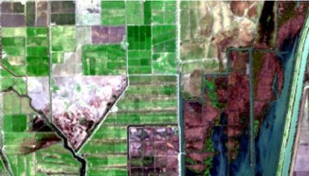
The idea is best described with images. Here is a display in mapview of an agricultural region in California’s Central Valley. The boundary of the region is a rectangle developed from UTM coordinates, and it is interesting that the boundary of the region is slightly tilted with respect to the network of roads and field boundaries. There are several possible explanations for this, but it does not affect our presentation, so we will ignore it.
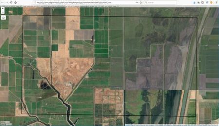 There are clearly several different cover types in the region, including fallow fields, planted fields, natural regions, and open water. Our objective is to develop a land classification of the region based on Landsat data. A common method of doing this is based on the so-called false color image. In a false color image, radiation in the green wavelengths is displayed as blue, radiation in the red wavelengths is displayed as green, and radiation in the infrared wavelengths is displayed as red. Here is a false color image of the region shown in the black rectangle.
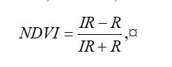
 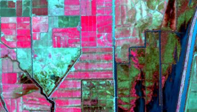 Because living vegetation strongly reflects radiation in the infrared region and absorbs it in the red region, the amount of vegetation contained in a pixel can be estimated by using the normalized difference vegetation index, or NDVI, defined as
 |
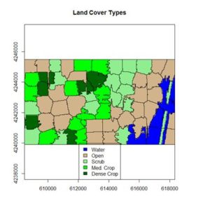
 If you compare the images you can see that the areas in black rectangle above that appear green have a high NDVI, the areas that appear brown have a low NDVI, and the open water in the southeast corner of the image actually has a negative NDVI, because water strongly absorbs infrared radiation. Our objective is to generate a classification of the land surface into one of five classes: dense vegetation, sparse vegetation, scrub, open land, and open water. Here is the classification generated using the method I am going to describe.
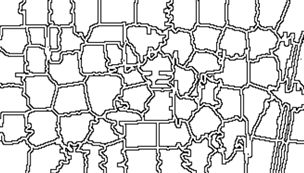
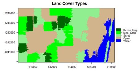 There are a number of image analysis packages available in R. I elected to use the OpenImageR and SuperpixelImageSegmentation packages, both of which were developed by L. Mouselimis (2018, 2019a). One reason for this choice is that the objects created by these packages have a very simple and transparent data structure that makes them ideal for data analysis and, in particular, for integration with the raster package. The packages are both based on the idea of image segmentation using superpixels . According to Stutz et al. (2018), superpixels were introduced by Ren and Malik (2003). Stutz et al. define a superpixel as “a group of pixels that are similar to each other in color and other low level properties.” Here is the false color image above divided into superpixels.
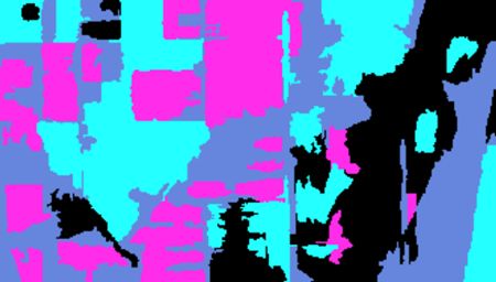
In the next section we will introduce the concepts of superpixel image segmentation and the application of these packages. In Section 3 we will discuss the use of these concepts in data analysis. The intent of image segmentation as implemented in these and other software packages is to provide support for human visualization. This can cause problems because sometimes a feature that improves the process of visualization detracts from the purpose of data analysis. In Section 4 we will see how the simple structure of the objects created by Mouselimis’s two packages can be used to advantage to make data analysis more powerful and flexible. This post is a shortened version of the Additional Topic that I described at the start of the post.
2. Introducing superpixel image segmentation
The discussion in this section is adapted from the R vignette Image Segmentation Based on Superpixels and Clustering (Mouselimis, 2019b). This vignette describes the R packages OpenImageR and SuperpixelImageSegmentation. In this post I will only discuss the OpenImageR package. It uses simple linear iterative clustering (SLIC, Achanta et al., 2010), and a modified version of this algorithm called SLICO (Yassine et al., 2018), and again for brevity I will only discuss the former. To understand how the SLIC algorithm works, and how it relates to our data analysis objective, we need a bit of review about the concept of color space. Humans perceive color as a mixture of the primary colors red, green, and blue (RGB), and thus a “model” of any given color can in principle be described as a vector in a three-dimensional vector space. The simplest such color space is one in which each component of the vector represents the intensity of one of the three primary colors. Landsat data used in land classification conforms to this model. Each band intensity is represented as an integer value between 0 and 255. The reason is that this covers the complete range of values that can be represented by a sequence of eight binary (0,1) values because 28 – 1 = 255. For this reason it is called the eight-bit RGB color model.
There are other color spaces beyond RGB, each representing a transformation for some particular purpose of the basic RGB color space. A common such color space is the CIELAB color space, defined by the International Commission of Illumination (CIE). You can read about this color space here. In brief, quoting from this Wikipedia article, the CIELAB color space “expresses color as three values: L* for the lightness from black (0) to white (100), a* from green (−) to red (+), and b* from blue (−) to yellow (+). CIELAB was designed so that the same amount of numerical change in these values corresponds to roughly the same amount of visually perceived change.”
Each pixel in an image contains two types of information: its color, represented by a vector in a three dimensional space such as the RGB or CIELAB color space, and its location, represented by a vector in two dimensional space (its x and y coordinates). Thus the totality of information in a pixel is a vector in a five dimensional space. The SLIC algorithm performs a clustering operation similar to K-means clustering on the collection of pixels as represented in this five-dimensional space.
The SLIC algorithm measures total distance between pixels as the sum of two components, dlab, the distance in the CIELAB color space, and dxy, the distance in pixel (x,y) coordinates. Specifically, the distance Ds is computed as
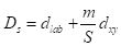 where S is the grid interval of the pixels and m is a compactness parameter that allows one to emphasize or de-emphasize the spatial compactness of the superpixels. The algorithm begins with a set of K cluster centers regularly arranged in the (x,y) grid and performs K-means clustering of these centers until a predefined convergence measure is attained.
The following discussion assumes some basic familiarity with the raster package. If you are not familiar with this package, an excellent introduction is given here. After downloading the data files, you can use them to first construct RasterLayer objects and then combine them into a RasterBrick.
library(raster)
> b2 <- raster(“region_blue.grd”)
> b3 <- raster(“region_green.grd”)
> b4 <- raster(“region_red.grd”)
> b5 <- raster(“region_IR.grd”)
> region.brick <- brick(b2, b3, b4, b5)
> print(nrows <- region.brick@nrows)
[1] 187
> print(ncols <- region.brick@ncols)
[1] 329
Next we plot the region.brick object (shown above) and write it to disk.
> # False color image
> plotRGB(region.brick, r = 4, g = 3, b = 2,
+ stretch = “lin”)
> # Write the image to disk
> jpeg(“FalseColor.jpg”, width = ncols,
+ height = nrows)
> plotRGB(region.brick, r = 4, g = 3, b = 2,
+ stretch = “lin”)
> dev.off()
We will now use SLIC for image segmentation. The code here is adapted directly from the superpixels vignette.
> library(OpenImageR)
> False.Color <- readImage(“FalseColor.jpg”)
> Region.slic = superpixels(input_image =
+ False.Color, method = “slic”, superpixel = 80,
+ compactness = 30, return_slic_data = TRUE,
+ return_labels = TRUE, write_slic = “”,
+ verbose = FALSE)
Warning message:
The input data has values between 0.000000 and 1.000000. The image-data will be multiplied by the value: 255!
> imageShow(Region.slic$slic_data)
We will discuss the warning message in Section 3. The function imageShow() is part of the OpenImageR package.
The OpenImageR function superpixels() creates superpixels, but it does not actually create an image segmentation in the sense that we are using the term is defined in Section 1. This is done by functions in the SuperPixelImageSegmentation package (Mouselimis, 2018), whose discussion is also contained in the superpixels vignette. This package is also described in the Additional Topic. As pointed out there, however, some aspects that make the function well suited for image visualization detract from its usefulness for data analysis, so we won’t discuss it further in this post. Instead, we will move directly to data analysis using the OpenImageR package.
3. Data analysis using superpixels
To use the functions in the OpenImageR package for data analysis, we must first understand the structure of objects created by these packages. The simple, open structure of the objects generated by the function superpixels() makes it an easy matter to use these objects for our purposes. Before we begin, however, we must discuss a preliminary matter: the difference between a Raster* object and a raster object. In Section 2 we used the function raster() to generate the blue, green, red and IR band objects b2, b3, b4, and b5, and then we used the function brick() to generate the object region.brick. Let’s look at the classes of these objects.
> class(b3)
[1] “RasterLayer”
attr(,”package”)
[1] “raster”
> class(full.brick)
[1] “RasterBrick”
attr(,”package”)
[1] “raster”
Objects created by the raster packages are called Raster* objects, with a capital “R”. This may seem like a trivial detail, but it is important to keep in mind because the objects generated by the functions in the OpenImageR and SuperpixelImageSegmentation packages are raster objects that are not Raster* objects (note the deliberate lack of a courier font for the word “raster”).
In Section 2 we used the OpenImageR function readImage() to read the image data into the object False.Color for analysis. Let’s take a look at the structure of this object.
> str(False.Color)
num [1:187, 1:329, 1:3] 0.373 0.416 0.341 0.204 0.165 …
It is a three-dimensional array, which can be thought of as a box, analogous to a rectangular Rubik’s cube. The “height” and “width” of the box are the number of rows and columns respectively in the image and at each value of the height and width the “depth” is a vector whose three components are the red, green, and blue color values of that cell in the image, scaled to [0,1] by dividing the 8-bit RGB values, which range from 0 to 255, by 255. This is the source of the warning message that accompanied the output of the function superpixels(), which said that the values will be multiplied by 255. For our purposes, however, it means that we can easily analyze images consisting of transformations of these values, such as the NDVI. Since the NDVI is a ratio, it doesn’t matter whether the RGB values are normalized or not. For our case the RasterLayer object b5 of the RasterBrick False.Color is the IR band and the object b4 is the R band. Therefore we can compute the NDVI as
> NDVI.region <- (b5 – b4) / (b5 + b4)
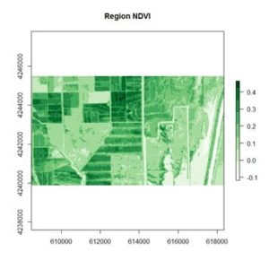
Since NDVI is a ratio scale quantity, the theoretically best practice is to plot it using a monochromatic representation in which the brightness of the color (i.e., the color value) represents the value (Tufte, 1983). We can accomplish this using the RColorBrewer function brewer.pal().> library(RColorBrewer)
> plot(NDVI.region, col = brewer.pal(9, “Greens”),
+ axes = TRUE, main = “Region NDVI”)
This generates the NDVI map shown above. The darkest areas have the highest NDVI. Let’s take a look at the structure of the RasterLayer object NDVI.region.
> str(NDVI.region)
Formal class ‘RasterLayer’ [package “raster”] with 12 slots
* * *
..@ data :Formal class ‘.SingleLayerData’ [package “raster”] with 13 slots
* * *
.. .. ..@ values : num [1:61523] 0.1214 0.1138 0.1043 0.0973 0.0883 …
* * *
..@ ncols : int 329
..@ nrows : int 187
Only the relevant parts are shown, but we see that we can convert the raster data to a matrix that can be imported into our image segmentation machinery as follows. Remember that by default R constructs matrices by columns. The data in Raster* objects such as NDVI.region are stored by rows, so in converting these data to a matrix we must specify byrow = TRUE.
> NDVI.mat <- matrix(NDVI.region@data@values,
+ nrow = NDVI.region@nrows,
+ ncol = NDVI.region@ncols, byrow = TRUE)
The function imageShow() works with data that are either in the eight bit 0 – 255 range or in the [0,1] range (i.e., the range of x between and including 0 and 1). It does not, however, work with NDVI values if these values are negative. Therefore, we will scale NDVI values to [0,1].
> m0 <- min(NDVI.mat)
> m1 <- max(NDVI.mat)
> NDVI.mat1 <- (NDVI.mat – m0) / (m1 – m0)
> imageShow(NDVI.mat)
Here is the resulting image.
The function imageShow() deals with a single layer object by producing a grayscale image. Unlike the green NDVI plot above, in this plot the lower NDVI regions are darker.
We are now ready to carry out the segmentation of the NDVI data. Since the structure of the NDVI image to be analyzed is the same as that of the false color image, we can simply create a copy of this image, fill it with the NDVI data, and run it through the superpixel image segmentation function. If an image has not been created on disk, it is also possible (see the Additional Topic) to create the input object directly from the data.
> NDVI.data <- False.Color
> NDVI.data[,,1] <- NDVI.mat1
> NDVI.data[,,2] <- NDVI.mat1
> NDVI.data[,,3] <- NDVI.mat1 In the next section we will describe how to create an image segmentation of the NDVI data and how to use cluster analysis to create a land classification.
4. Expanding the data analysis capacity of superpixels
Here is an application of the function superpixels() to the NDVI data generated in Section 3.
> NDVI.80 = superpixels(input_image = NDVI.data,
+ method = “slic”, superpixel = 80,
+ compactness = 30, return_slic_data = TRUE,
+ return_labels = TRUE, write_slic = “”,
+ verbose = FALSE)
> imageShow(Region.slic$slic_data)
Here is the result.
 Here the structure of the object NDVI.80 .
> str(NDVI.80)
List of 2
$ slic_data: num [1:187, 1:329, 1:3] 95 106 87 52 42 50 63 79 71 57 …
$ labels : num [1:187, 1:329] 0 0 0 0 0 0 0 0 0 0 …
It is a list with two elements, NDVI.80$slic_data, a three dimensional array of pixel color data (not normalized), and NDVI.80$labels, a matrix whose elements correspond to the pixels of the image. The second element’s name hints that it may contain values identifying the superpixel to which each pixel belongs. Let’s see if this is true.
> sort(unique(as.vector(NDVI.80$labels)))
[1] 0 1 2 3 4 5 6 7 8 9 10 11 12 13 14 15 16 17 18 19 20 21 22 23
[25] 24 25 26 27 28 29 30 31 32 33 34 35 36 37 38 39 40 41 42 43 44 45 46 47
[49] 48 49 50 51 52 53 54 55 56 57 58 59 60 61 62 63 64 65 66 67 68 69 70 71
There are 72 unique labels. Although the call to superpixels() specified 80 superpixels, the function generated 72. We can see which pixels have the label value 0 by setting the values of all of the other pixels to [255, 255, 255], which will plot as white.
> R0 <- NDVI.80
for (i in 1:nrow(R0$label))
+ for (j in 1:ncol(R0$label))
+ if (R0$label[i,j] != 0)
+ R0$slic_data[i,j,] <- c(255,255,255)
> imageShow(R0$slic_data)
This produces the plot shown here.
 The operation isolates the superpixel in the upper right corner of the image, together with the corresponding portion of the boundary. We can easily use this approach to figure out which value of NDVI.80$label corresponds to which superpixel. Now let’s deal with the boundary. A little exploration of the NDVI.80 object suggests that pixels on the boundary have all three components equal to zero. Let’s isolate and plot all such pixels by coloring all other pixels white.
> Bdry <- NDVI.80
for (i in 1:nrow(Bdry$label))
+ for (j in 1:ncol(Bdry$label))
+ if (!(Bdry$slic_data[i,j,1] == 0 &
+ Bdry$slic_data[i,j,2] == 0 &
+ Bdry$slic_data[i,j,3] == 0))
+ Bdry$slic_data[i,j,] <- c(255,255,255)
> Bdry.norm <- NormalizeObject(Bdry$slic_data)
> imageShow(Bdry$slic_data)
This shows that we have indeed identified the boundary pixels. Note that the function imageShow() displays these pixels as white with a black edge, rather than pure black. Having done a preliminary analysis, we can organize our segmentation process into two steps. The first step will be to replace each of the superpixels generated by the OpenImageR function superpixels() with one in which each pixel has the same value, corresponding to a measure of central tendency (e.g, the mean, median , or mode) of the original superpixel. The second step will be to use the K-means unsupervised clustering procedure to organize the superpixels from step 1 into a set of clusters and give each cluster a value corresponding to a measure of central tendency of the cluster. I used the code developed to identify the labels and to generate the boundary to construct a function make.segments() to carry out the segmentation. The first argument of make.segments() is the superpixels object, and the second is the functional measurement of central tendency. Although in this case each of the three colors of the object NDVI.80 have the same values, this may not be true for every application, so the function analyzes each color separately. Because the function is rather long, I have not included it in this post. If you want to see it, you can go to the Additional Topic linked to the book’s website.
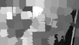
Here is the application of the function to the object NDVI.80 with the second argument set to mean.
> NDVI.means <- make.segments(NDVI.80, mean)
> imageShow(NDVI.means$slic_data)
Here is the result.
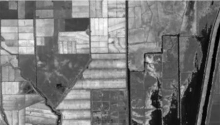
The next step is to develop clusters that represent identifiable land cover types. In a real project the procedure would be to collect a set of ground truth data from the site, but that option is not available to us. Instead we will work with the true color rendition of the Landsat scene, shown here.
 The land cover is subdivided using K-means into five types: dense crop, medium crop, scrub, open, and water.
> NDVI.clus <-
+ kmeans(as.vector(NDVI.means$slic_data[,,1]), 5)
> vege.class <- matrix(NDVI.clus$cluster,
+ nrow = NDVI.region@nrows,
+ ncol = NDVI.region@ncols, byrow = FALSE)
> class.ras <- raster(vege.class, xmn = W,
+ xmx = E, ymn = S, ymx = N, crs =
+ CRS(“+proj=utm +zone=10 +ellps=WGS84”))
Next I used the raster function ratify() to assign descriptive factor levels to the clusters.
> class.ras <- ratify(class.ras)
> rat.class <- levels(class.ras)[[1]]
> rat.class$landcover <- c(“Water”, “Open”,
+ “Scrub”, “Med. Crop”, “Dense Crop”)
> levels(class.ras) <- rat.class
> levelplot(class.ras, margin=FALSE,
+ col.regions= c(“blue”, “tan”,
+ “lightgreen”, “green”, “darkgreen”),
+ main = “Land Cover Types”)
The result is shown in the figure at the start of the post. We can also overlay the original boundaries on top of the image. This is more easily done using plot() rather than levelplot(). The function plot() allows plots to be built up in a series of statements. The function levelplot() does not.
> NDVI.rasmns <- raster(NDVI.means$slic_data[,,1],
+ xmn = W, xmx = E, ymn = S, ymx = N,
+ crs = CRS(“+proj=utm +zone=10 +ellps=WGS84”))
> NDVI.polymns <- rasterToPolygons(NDVI.rasmns,
+ dissolve = TRUE)
> plot(class.ras, col = c(“blue”, “tan”,
+ “lightgreen”, “green”, “darkgreen”),
+ main = “Land Cover Types”, legend = FALSE)
> legend(“bottom”, legend = c(“Water”, “Open”,
+ “Scrub”, “Med. Crop”, “Dense Crop”),
+ fill = c(“blue”, “tan”, “lightgreen”, “green”,
+ “darkgreen”))
> plot(NDVI.polymns, add = TRUE)
The application of image segmentation algorithms to remotely sensed image classification is a rapidly growing field, with numerous studies appearing every year. At this point, however, there is little in the way of theory on which to base an organization of the topic. If you are interested in following up on the subject, I encourage you to explore it on the Internet.
References
Achanta, R., A. Shaji, K. Smith, A. Lucchi, P. Fua, and S. Susstrunk (2010). SLIC Superpixels. Ecole Polytechnique Fedrale de Lausanne Technical Report 149300.
Appelhans, T., F. Detsch, C. Reudenbach and S. Woellauer (2017). mapview: Interactive Viewing of Spatial Data in R. R package version 2.2.0. https://CRAN.R-project.org/package=mapview Bivand, R., E. Pebesma, and V. Gómez-Rubio. (2008). Applied Spatial Data Analysis with R. Springer, New York, NY.
Frey, B.J. and D. Dueck (2006). Mixture modeling by affinity propagation. Advances in Neural Information Processing Systems 18:379.
Hijmans, R. J. (2016). raster: Geographic Data Analysis and Modeling. R package version 2.5-8. https://CRAN.R-project.org/package=raster
Mouselimis, L. (2018). SuperpixelImageSegmentation: Superpixel Image Segmentation. R package version 1.0.0. https://CRAN.R-project.org/package=SuperpixelImageSegmentation
Mouselimis, L. (2019a). OpenImageR: An Image Processing Toolkit. R package version 1.1.5. https://CRAN.R-project.org/package=OpenImageR
Mouselimis, L. (2019b) Image Segmentation Based on Superpixel Images and Clustering. https://cran.r-project.org/web/packages/OpenImageR/vignettes/Image_segmentation_superpixels_clustering.html.
Ren, X., and J. Malik (2003) Learning a classification model for segmentation. International Conference on Computer Vision, 2003, 10-17.
Stutz, D., A. Hermans, and B. Leibe (2018). Superpixels: An evaluation of the state-of-the-art. Computer Vision and Image Understanding 166:1-27.
Tufte, E. R. (1983). The Visual Display of Quantitative Information. Graphics Press, Cheshire, Conn.
Yassine, B., P. Taylor, and A. Story (2018). Fully automated lung segmentation from chest radiographs using SLICO superpixels. Analog Integrated Circuits and Signal Processing 95:423-428.
Zhou, B. (2013) Image segmentation using SLIC superpixels and affinity propagation clustering. International Journal of Science and Research. https://pdfs.semanticscholar.org/6533/654973054b742e725fd433265700c07b48a2.pdf
 And finally, we will show the randomness line; in order to do that:
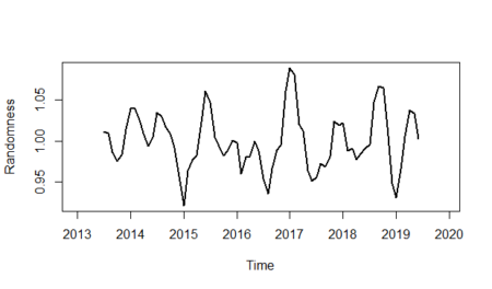


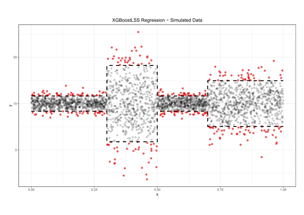
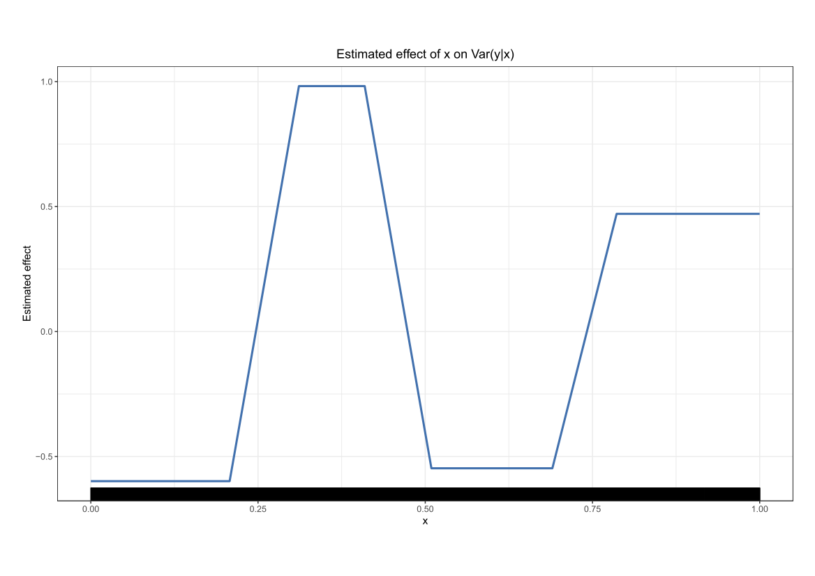
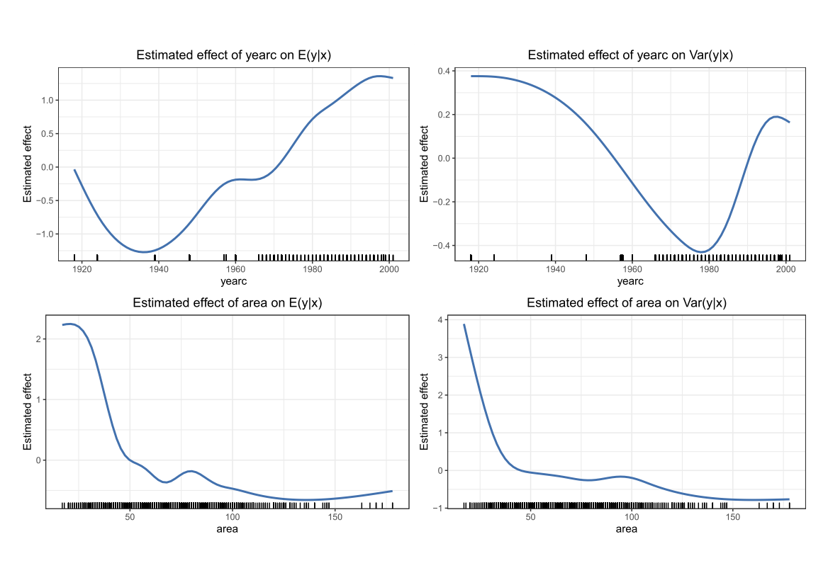
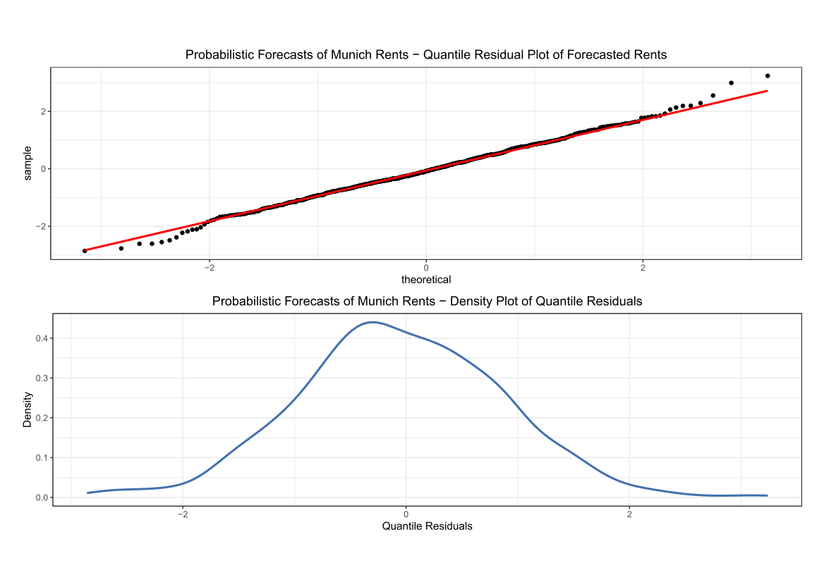
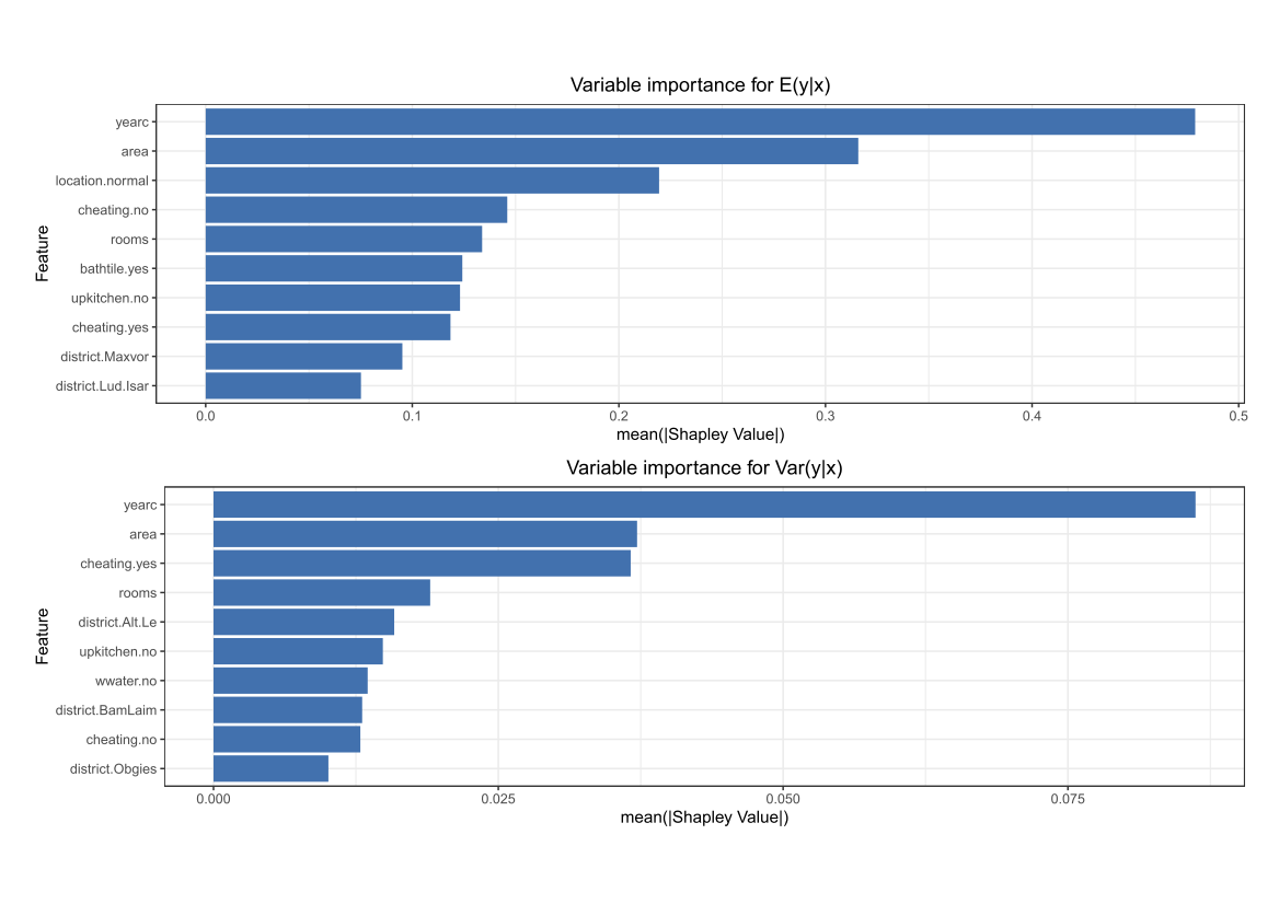
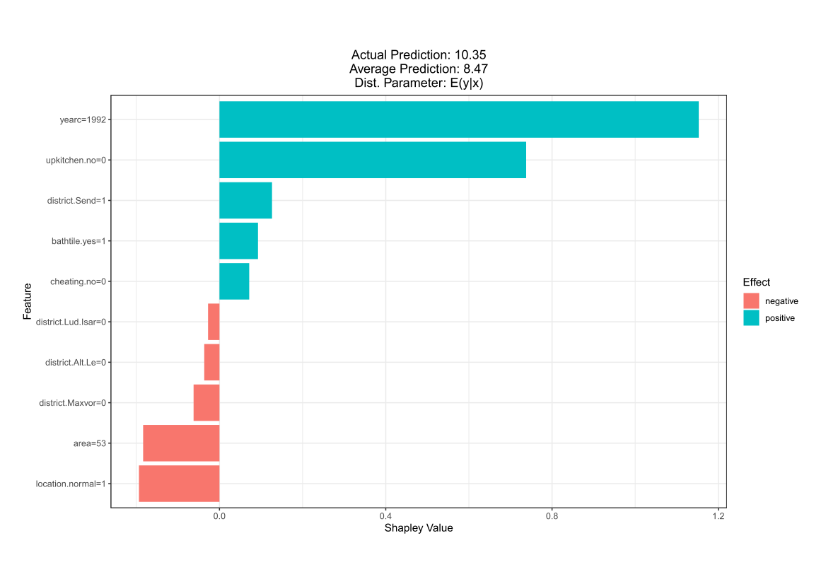
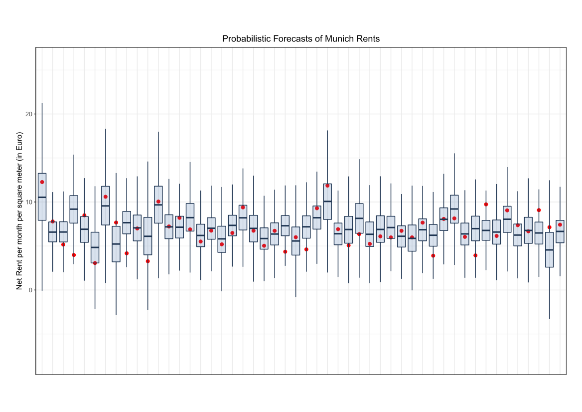
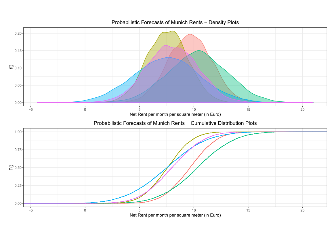
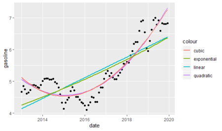
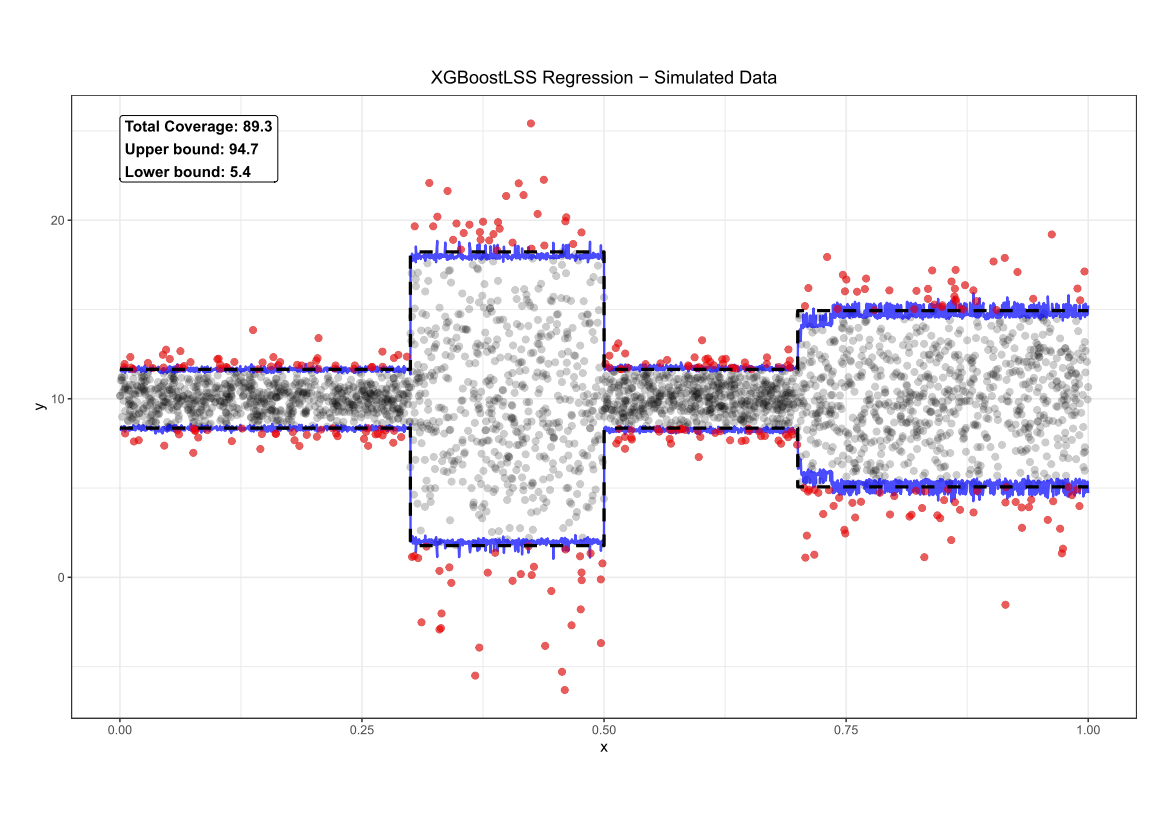 Comparing the coverage of the intervals with the nominal level of 90% shows that XGBoostLSS does not only correctly model the heteroskedasticity in the data, but it also provides an accurate forecast for the 5% and 95% quantiles. The flexibility of XGBoostLSS also comes from its ability to provide attribute importance, as well as partial dependence plots, for all of the distributional parameters.