Natural Gas Prices Are Again on an Unsustainable Upward Trajectory …

Interested in publishing a one-time post on R-bloggers.com? Press here to learn how.

I identified a real-time market condition in the natural gas market (symbol = UNG) on LinkedIn and followed up on a prior r-bloggers post here. The market ultimately declined 42% following the earlier breach of its identified unsustainable Stealth Support Curve.

Chart from earlier r-blogger post

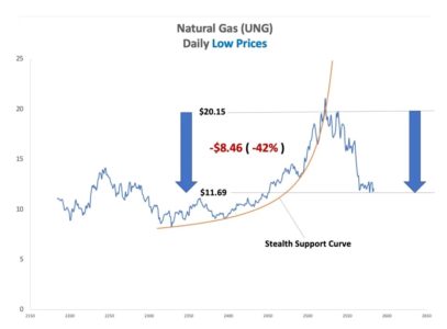
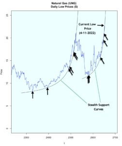
In short order, this same market is once again on another such path. Once this market meaningfully breaks its current Stealth Support Curve, the magnitude of its ultimate decline is naturally indeterminate and is in no way guaranteed to again be ‘large.’ Nonetheless, it is highly improbable for market price evolution to continue along its current trajectory. If market low prices continue to adhere to the current Stealth Support Curve (below), prices will increase at least +1,800% within a month. Thus, the forecast of impending Stealth Support Curve breach is not a difficult one. The relevant questions are 1) when will it occur and 2 ) what is the magnitude of decline following the breach?

Past and Current Stealth Support Curves

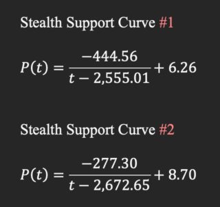
Stealth Support Curve Formulas

t1 = 9/28/2011

R Code

library(tidyverse)
library(readxl)

# Original data source - https://www.nasdaq.com/market-activity/funds-and-etfs/ung/historical

# Download reformatted data (columns/headings) from my github site and save to a local drive

# https://github.com/123blee/Stealth_Curves.io/blob/main/UNG_prices_4_11_2022.xlsx

# Load your local data file
ung <- read_excel("... Insert your local file path here .../UNG_prices_4_11_2022.xlsx")
ung


# Convert 'Date and Time' to 'Date' column
ung[["Date"]] <- as.Date(ung[["Date"]])
ung

bars <- nrow(ung)

# Add bar indicator as first tibble column
ung %
  add_column(t = 1:nrow(ung), .before = "Date")
ung

# Add 40 future days to the tibble for projection of the Stealth Curve once added
future <- 40
ung %
  add_row(t = (bars+1):(bars+future))

# Market Pivot Lows using 'Low' Prices
# Chart 'Low' UNG prices
xmin <- 2250
xmax <- bars + future
ymin <- 0
ymax <- 25
plot.new()
background <- c("azure1")
chart_title_low <- c("Natural Gas (UNG) \nDaily Low Prices ($)")
u <- par("usr") 
rect(u[1], u[3], u[2], u[4], col = background) 
par(ann=TRUE)
par(new=TRUE)
t <- ung[["t"]]
Price <- ung[["Low"]]
plot(x=t, y=Price, main = chart_title_low, type="l", col = "blue", 
     
     ylim = c(ymin, ymax) ,
     
     xlim = c(xmin, xmax ) ) 

# Add 1st Stealth Support Curve to tibble
# Stealth Support Curve parameters
a <-   -444.56  
b <-      6.26  
c <-  -2555.01  

ung %
  mutate(Stealth_Curve_Low_1 = a/(t + c) + b)
ung

# Omit certain Stealth Support Curve values from charting
ung[["Stealth_Curve_Low_1"]][1:2275] <- NA
ung[["Stealth_Curve_Low_1"]][2550:xmax] <- NA
ung

# Add 1st Stealth Curve to chart
lines(t, ung[["Stealth_Curve_Low_1"]])

# Add 2nd Stealth Support Curve to tibble
# Stealth Support Curve parameters
a <-   -277.30  
b <-      8.70  
c <-  -2672.65 

ung %
  mutate(Stealth_Curve_Low_2 = a/(t + c) + b)
ung

# Omit certain Stealth Support Curve values from charting
ung[["Stealth_Curve_Low_2"]][1:2550] <- NA
ung[["Stealth_Curve_Low_2"]][2660:xmax] <- NA
ung

# Add 2nd Stealth Curve to chart
lines(t, ung[["Stealth_Curve_Low_2"]])

The current low price is $22.68 on 4-11-2022 (Market close = $23.30).

The contents of this article are in no way meant to imply trading, investing, and/or hedging advice. Consult your personal financial expert(s) for all such matters. Details of Stealth Curve parameterization are found in my Amazon text, ‘Stealth Curves: The Elegance of Random Markets’ .

Brian K. Lee, MBA, PRM, CMA, CFA

Connect with me on LinkedIn.

Leave a Reply Cancel reply