This represents
Part 4 of a
4-part series relative to the calculation of
Equity Cash Flow (
ECF) using
R. If you missed any of the prior posts, be certain to reference them before proceeding. Content in this section builds on previously described information/data.
Part 3 of
4 prior post is located here –
Part 3 of 4 .
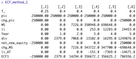
‘ECF – Method 4’ differs slightly from the prior 3 versions. Specifically, it represents ECF with an
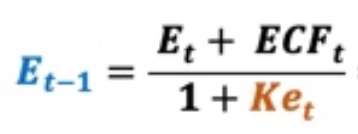
adjustment. By definition, Equity Value (
E) is calculated as the present value of a series of Equity Cash Flow (
ECF) discounted at the appropriate discount rate, the cost of levered equity capital,
Ke. When using forward rate discounting, the equation for
E is as follows:
The cost of levered equity capital (Ke) is shown below.
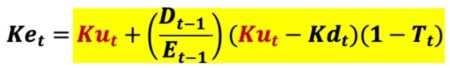
Where
Many DCF practitioners
incorrectly assume the cost of equity capital (
Ke) is
constant in all periods. The above equation indicates
Ke can easily vary over time even if
Ku,
Kd, and
T are all
constant values. Assuming a constant
Ke value when such does not apply violates a basic premise of valuation, the
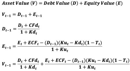
value additivity rule, Debt Value (
D) + Equity Value (
E) = Asset Value (
V).
Substituting the cost of equity capital (
Ke) into the Equity valuation (
E) equation yield this.
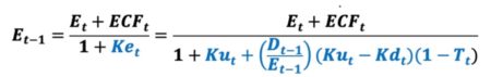
Note in the above valuation equation, equity value is a function of itself. We require Equity Value (
E) in the prior period (t-1) in order to obtain the discount rate (
Ke) for the current period “t.” This current period discount rate is used to calculate prior period’s equity value. This is clearly a circular calculation, as Equity Value (
E) in the prior period (t-1) exists on both sides of the equation. While Excel solutions with intentional circular references such as this can be problematic, R experiences no such problems in proper iterative solution.
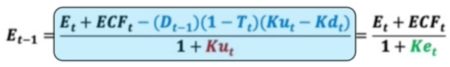
Even so, we can completely bypass calculation circularity altogether and arrive at the correct iterative, circular solution. Using simple 8
th grade math, a noncircular equity valuation equation is derived. Note this new noncircular equation requires a noncircular discount rate (
Ku) and a noncircular numerator term in which to discount. All calculation circularity is eliminated in the equity valuation equation. The numerator includes a noncircular adjustment to Equity Cash Flow (
ECF).
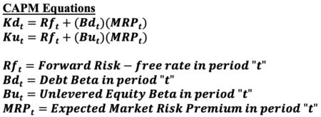
The 2 noncircular discount rates (
Ku,
Kd) are calculated using the Capital Asset Pricing Model (
CAPM).
The noncircular debt valuation (
D) equation using forward rate (
Kd) discounting is provided below.
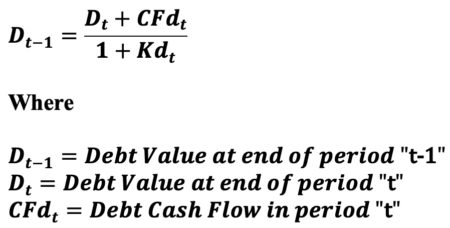
Reference Part
2 of
4 in this series for the calculation of debt cash flow (
CFd).
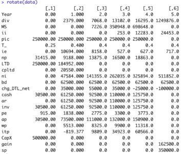
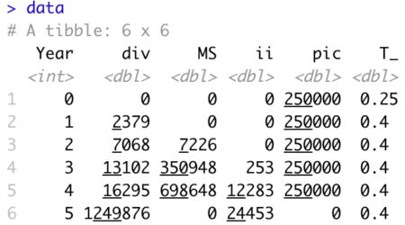
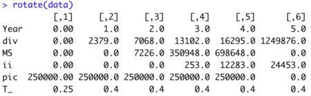
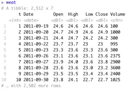
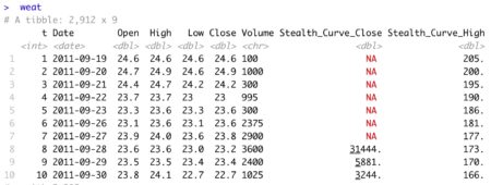
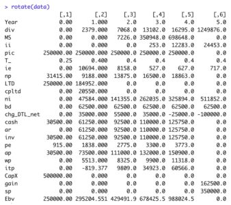
Update ‘data’ tibble
data <- data %>%
  mutate(Rf = rep(0.03, 6),
         MRP = rep(0.04, 6),
         Bd = rep(0.2, 6),
         Bu = rep(1.1, 6),
         Kd = Rf + Bd * MRP,
         Ku = Rf + Bu * MRP,
         N = np + cpltd + LTD,   # All interest bearing debt
         CFd = ie - (N - lag(N, default=0)),
         ECF3 = ni - ii*(1-T_) - ( Ebv - lag(Ebv, default=0) ) + ( MS  - lag(MS, default=0)) )
View tibble
rotate(data)
The R code below calculates Debt Value (
D) and Equity Value (
E) each period. The function sum these 2 values to obtain asset value (
V).
R Code – ‘valuation’ R function
valuation <- function(a) {

  library(tidyverse)

  n <- length(a$bd) - 1

  Rf  <- a$Rf
  MRP <- a$MRP
  Ku  <- a$Ku
  Kd  <- a$Kd
  T_   <- a$T_

  # Flow values

  CFd <- a$CFd
  ECF <- a$ECF3

  # Initialize valuation vectors to zero by Year

  d <- rep(0, n+1 )  # Initialize debt value to zero each Year
  e <- rep(0, n+1 )  # Initialize equity value to zero each Year

  # Calculate debt and equity value by period in reverse order using discount rates 'Kd' and 'Ku', repsectively

  for (t in (n+1):2)    # reverse step through loop from period 'n+1' to 2
  {

    # Debt Valuation discounting 1-period at the forward discount rate, Kd[t]

    d[t-1] <- ( d[t] + CFd[t] ) / (1 + Kd[t] )

     # Equity Valuation discounting 1-period at the forward discount rate, Ku[t]

    e[t-1] <- ( e[t] + ECF[t] - (d[t-1])*(Ku[t]-Kd[t])*(1-T_[t]) ) / (1 + Ku[t] )

  }

  # Asset valuation by Year (Using Value Additivity Equation)
  v = d + e

  npv_0 <- round(e[1],0) + round(ECF[1],0)
  npv_0 <- c(npv_0, rep(NaN,n) )

  valuation <- as_tibble( cbind(a$Year, T_, Rf, MRP, Ku, Kd, Ku-Kd, ECF,
                                   -lag(d, default=0)*(1-T_)*(Ku-Kd), ECF - lag(d, default=0)*(1-T_)*(Ku-Kd),
                                    d, e, v, d/e, c( ECF[1], rep(NaN,n)), npv_0 ) )

  names(valuation) <- c("Year", "T", "Rf", "MRP", "Ku", "Kd", "Ku_Kd", "ECF",
                           "ECF_adj", "ADJ_ECF", "D", "E", "V", "D_E_Ratio", "ECF_0", "NPV_0")

  return(rotate(valuation))
}
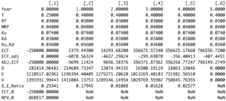
View R output
valuation <- valuation( data )

round(valuation, 5)
This method of noncircular equity valuation (
E) is simple and straightforward. Unfortunately, DCF practitioners tend to incorrectly treat
Ke as a noncircular calculation using CAPM. That widely used approach violates the
value additivity rule.
Additionally, there is a widely held belief the Adjusted Present Value (
APV) asset valuation approach is the only one that provides a means of calculating asset value in a noncircular fashion.
Citation: Fernandez, Pablo, (August 27, 2020),
Valuing Companies by Cash Flow Discounting: Only APV Does Not Require Iteration.
Though the
APV method is almost 50 years old, there is little agreement as to how to correctly calculate one of the model’s 2 primary components – the value of interest expense tax shields. The above 8
th grade approach to equity valuation (
E) eliminates the need to use the
APV model for asset valuation if calculation by noncircular means is the goal.
Simply sum the 2 noncircular valuation equations below (
D + E). They ensure the enforcement of the
value-additivity rule (
V = D + E).
Valuation Additivity Rule
(Assuming debt and equity are the 2 sources of financing)
In summary,
circular equity valuation (
E) is entirely
eliminated using simple
8th grade math.
Adding this
noncircular equity valuation (
E) solution to
noncircular debt valuation (
D) results in
noncircular asset valuation (
V).
There is no need to further academically squabble over the correct methodology for valuing tax shields relative to the
noncircular APV asset valuation model. Tax shields are not separately discounted using the above approach.
This example is taken from my newly published textbook, ‘
Advanced Discounted Cash Flow (DCF) Valuation using R.’ The above method is discussed in far greater detail, including the requisite 8
th grade math, along with development of the integrated financials using
R. Included in the text are
40+ advanced
DCF valuation models – all of which are
value-additivity compliant.
Typical corporate finance texts do
not teach this very important concept. As a result, DCF practitioners often unknowingly violate the immensely important
value-additivity rule. This modeling error is closely akin to violating the
accounting equation (Book Assets = Book Liabilities + Book Equity) when constructing pro form balance sheets used in a DCF valuation.
For some reason, violation of the
accounting equation is considered a valuation sin, while violation of the
value-additivity rule is a well-established practice in DCF valuation land.
Reference my website for additional details.
https://www.leewacc.com/
Next up, 10 Different, Mathematically Equivalent Ways to Calculate Free Cash Flow (FCF) …
Brian K. Lee, MBA, PRM, CMA, CFA
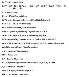
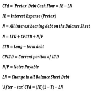
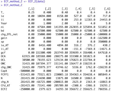
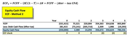
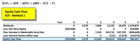
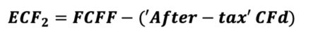 The equation appears innocent enough, though there are many underlying terms that require definition for understanding of the calculation. In words, ‘ECF – Method 2’ equals free cash Flow (FCFF) minus after-tax Debt Cash Flow (CFd).