Gauging Cryptocurrency Market Sentiment in R

Navigating the volatile world of cryptocurrencies requires a keen understanding of market sentiment. This blog post explores some of the essential tools and techniques for analyzing the mood of the crypto market, using the cryptoQuotes-package.

The Cryptocurrency Fear and Greed Index in R

The Fear and Greed Index is a market sentiment tool that measures investor emotions, ranging from 0 (extreme fear) to 100 (extreme greed). It analyzes data like volatility, market momentum, and social media trends to indicate potential overvaluation or undervaluation of cryptocurrencies. This index helps investors identify potential buying or selling opportunities by gauging the market’s emotional extremes.

This index can be retrieved by using the cryptoQuotes::getFGIndex()-function, which returns the daily index within a specified time-frame,

## Fear and Greed Index
## from the last 14 days
tail(
  FGI <- cryptoQuotes::getFGIndex(
    from = Sys.Date() - 14
  )
)
#>            FGI
#> 2024-01-03  70
#> 2024-01-04  68
#> 2024-01-05  72
#> 2024-01-06  70
#> 2024-01-07  71
#> 2024-01-08  71

The Long-Short Ratio of a Cryptocurrency Pair in R

The Long-Short Ratio is a financial metric indicating market sentiment by comparing the number of long positions (bets on price increases) against short positions (bets on price decreases) for an asset. A higher ratio signals bullish sentiment, while a lower ratio suggests bearish sentiment, guiding traders in making informed decisions.

The Long-Short Ratio can be retrieved by using the cryptoQuotes::getLSRatio()-function, which returns the ratio within a specified time-frame and granularity. Below is an example using the Daily Long-Short Ratio on Bitcoin (BTC),

## Long-Short Ratio
## from the last 14 days
tail(
  LSR <- cryptoQuotes::getLSRatio(
    ticker = "BTCUSDT",
    interval = '1d',
    from = Sys.Date() - 14
  )
)
#>              Long  Short LSRatio
#> 2024-01-03 0.5069 0.4931  1.0280
#> 2024-01-04 0.6219 0.3781  1.6448
#> 2024-01-05 0.5401 0.4599  1.1744
#> 2024-01-06 0.5499 0.4501  1.2217
#> 2024-01-07 0.5533 0.4467  1.2386
#> 2024-01-08 0.5364 0.4636  1.1570

Putting it all together

Even though cryptoQuotes::getLSRatio() is an asset-specific sentiment indicator, and cryptoQuotes::getFGIndex() is a general sentiment indicator, there is much information to be gathered by combining this information.

This information can be visualized by using the the various charting-functions in the cryptoQuotes-package,

## get the BTCUSDT
## pair from the last 14 days
BTCUSDT <- cryptoQuotes::getQuote(
  ticker = "BTCUSDT",
  interval = "1d",
  from = Sys.Date() - 14
)
## chart the BTCUSDT
## pair with sentiment indicators
cryptoQuotes::chart(
  slider = FALSE,
  chart = cryptoQuotes::kline(BTCUSDT) %>%
    cryptoQuotes::addFGIndex(FGI = FGI) %>% 
    cryptoQuotes::addLSRatio(LSR = LSR)
)
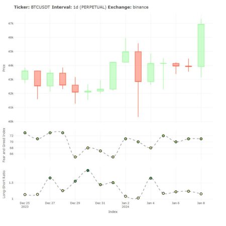
Bitcoin charted against Fear and Greed Index and the Long-Short Ratio using R
Bitcoin (BTC) plotted with Fear and Greed Index along side the Long-Short Ratio

Installing cryptoQuotes

Installing via CRAN

# install from CRAN
install.packages(
  pkgs = 'cryptoQuotes',
  dependencies = TRUE
)

Installing via Github

# install from github
devtools::install_github(
  repo = 'https://github.com/serkor1/cryptoQuotes/',
  ref = 'main'
)

Note: The latest price may vary depending on time of publication relative to the rendering time of the document. This document were rendered at 2024-01-08 23:30 CET

Cryptocurrency Market Data in R

Getting cryptocurrency OHLCV data in R without having to depend on low-level coding using, for example, curl or httr2, have not been easy for the R community.

There is now a high-level API Client available on CRAN which fetches all the market data without having to rely on web-scrapers, API keys or low-level coding.

Bitcoin Prices in R (Example)

This high-level API-client have one main function, getQuotes(), which returns cryptocurrency market data with a xts– and zoo-class. The returned objects contains Open, High, Low, Close and Volume data with different granularity, from the currently supported exchanges.

In this blog post I will show how to get hourly Bitcoin (BTC) prices in R
using the getQuotes()-function. See the code below,
# 1) getting hourly BTC
# from the last 3 days

BTC <- cryptoQuotes::getQuote(
 ticker   = "BTCUSDT", 
 source   = "binance", 
 futures  = FALSE, 
 interval = "1h", 
 from     = as.character(Sys.Date() - 3)
)
Bitcoin (BTC) OHLC-prices (Output from getQuote-function)
Index Open High Low Close Volume
2023-12-23 19:00:00 43787.69 43821.69 43695.03 43703.81 547.96785
2023-12-23 20:00:00 43703.82 43738.74 43632.77 43711.33 486.4342
2023-12-23 21:00:00 43711.33 43779.71 43661.81 43772.55 395.6197
2023-12-23 22:00:00 43772.55 43835.94 43737.85 43745.86 577.03505
2023-12-23 23:00:00 43745.86 43806.38 43701.1 43702.16 940.55167
2023-12-24 43702.15 43722.25 43606.18 43716.72 773.85301

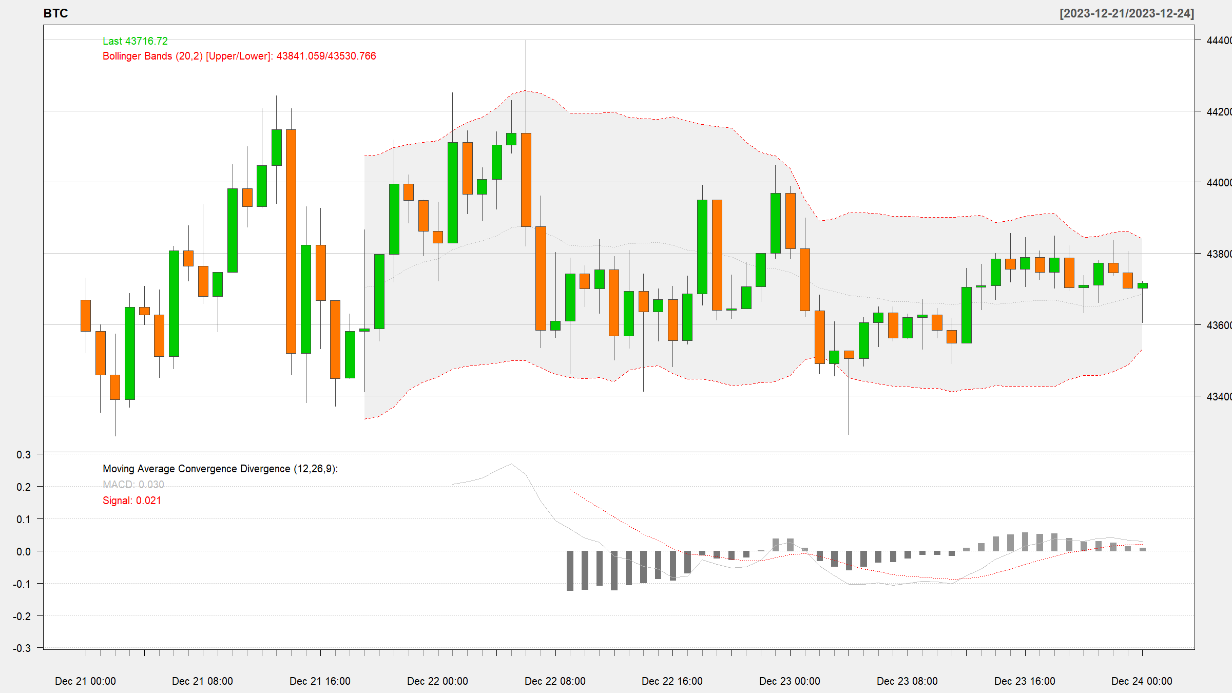
The returned Bitcoin prices from getQuotes() are compatible with quantmod and TTR, without further programming. Let me demonstrate this using chartSeries(), addBBands() and addMACD() from these powerful libraries,

# charting BTC
# using quantmod
quantmod::chartSeries(
 x = BTC,
 TA = c(
    # add bollinger bands
    # to the chart
    quantmod::addBBands(), 
    # add MACD indicator
    # to the chart
    quantmod::addMACD()
 ), 
 theme = quantmod::chartTheme("white")
)
Cryptocurrency charts using R
Charting Bitcoin prices using quantmod and TTR

Installing cryptoQuotes

Stable version

# install from CRAN
install.packages(
  pkgs = 'cryptoQuotes',
  dependencies = TRUE
)

Development version

# install from github
devtools::install_github(
  repo = 'https://github.com/serkor1/cryptoQuotes/',
  ref = 'main'
)

Using ChatGPT for Exploratory Data Analysis with Python, R and prompting

Join our workshop on Using ChatGPT for Exploratory Data Analysis with Python, R and prompting, which is a part of our workshops for Ukraine series! 


Here’s some more info: 


Title:Using ChatGPT for Exploratory Data Analysis with Python, R and prompting


Date: Thursday, November 30th, 18:00 – 20:00 CET (Rome, Berlin, Paris timezone)


Speaker: Gábor Békés is an Associate Professor at the Department of Economics and Business of Central European University, a research fellow at KRTK in Hungary, and a research affiliate at CEPR. His research is focused on international economics; economic geography and applied IO, and was published among others by the Global Strategy Journal, Journal of International Economics, Regional Science and Urban Economics or Economic Policy and have authored commentary on VOXEU.org. His comprehensive textbook, Data Analysis for Business, Economics, and Policy with Gábor Kézdi was publsihed by Cambridge University Press in 2021. 


Description: How can GenAI, like ChatGPT augment and speed up data exploration? Is it true that we no longer need coding skills? Or, instead, does ChatGPT hallucinate too much to be taken seriously? I will do a workshop with live prompting and coding to investigate.  I will experiment with two datasets shared ahead of the workshop.  The first comes from my Data Analysis textbook and is about football managers. Here I’ll see how close working with AI will get to what we have in the textbook, and compare codes written by us vs the machine. Second, I’ll work with a dataset I have no/little experience with and see how far it takes me. In this case, we will look at descriptive statistics, make graphs and tables, and work to improve a textual variable.  It will generate code and reports, and I’ll then check them on my laptop to see if they work. The process starts with Python but then I’ll proceed with R.


Minimal registration fee: 20 euro (or 20 USD or 800 UAH)


How can I register?


  • Save your donation receipt (after the donation is processed, there is an option to enter your email address on the website to which the donation receipt is sent)

  • Fill in the registration form, attaching a screenshot of a donation receipt (please attach the screenshot of the donation receipt that was emailed to you rather than the page you see after donation).

If you are not personally interested in attending, you can also contribute by sponsoring a participation of a student, who will then be able to participate for free. If you choose to sponsor a student, all proceeds will also go directly to organisations working in Ukraine. You can either sponsor a particular student or you can leave it up to us so that we can allocate the sponsored place to students who have signed up for the waiting list.


How can I sponsor a student?


  • Save your donation receipt (after the donation is processed, there is an option to enter your email address on the website to which the donation receipt is sent)

  • Fill in the sponsorship form, attaching the screenshot of the donation receipt (please attach the screenshot of the donation receipt that was emailed to you rather than the page you see after the donation). You can indicate whether you want to sponsor a particular student or we can allocate this spot ourselves to the students from the waiting list. You can also indicate whether you prefer us to prioritize students from developing countries when assigning place(s) that you sponsored.


If you are a university student and cannot afford the registration fee, you can also sign up for the waiting list here. (Note that you are not guaranteed to participate by signing up for the waiting list).


You can also find more information about this workshop series,  a schedule of our future workshops as well as a list of our past workshops which you can get the recordings & materials here.


Looking forward to seeing you during the workshop!


Visualising connection in R workshop

Join our workshop on Visualising connection in R, which is a part of our workshops for Ukraine series! 

Here’s some more info: 

Title: Visualising connection in R
Date: Thursday, November 9th, 19:00 – 21:00 CEST (Rome, Berlin, Paris timezone)
Speaker: Rita Giordano is a freelance data visualisation consultant and scientific illustrator based in the UK. By training, she is a physicist who holds a PhD in statistics applied to structural biology. She has extensive experience in research and data science. Furthermore, she has over fourteen years of professional experience working with R. She is also a LinkedIn instructor. You can find her course “Build Advanced Charts with R” on LinkedIn Learning.
Description: How to show connection? It depends on the connection we want to visualise. We could use a network, chord, or Sankey diagram.  The workshop will focus on how to visualise connections using chord diagrams. We will explore how to create a chord diagram with the {circlize} package.  In the final part of the workshop, I will briefly mention how to create a Sankey diagram with networkD3. Attendees need to have installed the {circlize} and {networkD3} packages.  
Minimal registration fee: 20 euro (or 20 USD or 800 UAH)


How can I register?


  • Save your donation receipt (after the donation is processed, there is an option to enter your email address on the website to which the donation receipt is sent)
  • Fill in the registration form, attaching a screenshot of a donation receipt (please attach the screenshot of the donation receipt that was emailed to you rather than the page you see after donation).

If you are not personally interested in attending, you can also contribute by sponsoring a participation of a student, who will then be able to participate for free. If you choose to sponsor a student, all proceeds will also go directly to organisations working in Ukraine. You can either sponsor a particular student or you can leave it up to us so that we can allocate the sponsored place to students who have signed up for the waiting list.


How can I sponsor a student?

  • Save your donation receipt (after the donation is processed, there is an option to enter your email address on the website to which the donation receipt is sent)
  • Fill in the sponsorship form, attaching the screenshot of the donation receipt (please attach the screenshot of the donation receipt that was emailed to you rather than the page you see after the donation). You can indicate whether you want to sponsor a particular student or we can allocate this spot ourselves to the students from the waiting list. You can also indicate whether you prefer us to prioritize students from developing countries when assigning place(s) that you sponsored.

If you are a university student and cannot afford the registration fee, you can also sign up for the waiting list here. (Note that you are not guaranteed to participate by signing up for the waiting list).


You can also find more information about this workshop series,  a schedule of our future workshops as well as a list of our past workshops which you can get the recordings & materials here.


Looking forward to seeing you during the workshop!


EARL your way: book your tickets now!

Your EARL tickets are now live to purchase here. Offering you every possible EARL ticket combination, here is a quick summary of what you can expect. You can simply choose a 3-day jam-packed conference pass or a 1 or 2-day option to customise an itinerary that works for you.

Grab your EARLy bird tickets right away – limited for a period of 2 weeks and 2 weeks only, we are delighted to be offering an unlimited amount of tickets ranging from 15-25% discount on all ticket options, depending if you are NHS, not for profit or an academic.

Team networking.

Why not bring your colleagues along for a much needed team social at the largest commercial R event in the UK? Offering lots of networking opportunities from brands in similar markets – there will be plenty of time to swap market experiences, over coffee, at lunch or at our evening reception. We are certainly proud to be a part of such an enthusiastic community.

Full or half day workshop on day 1.

We are running a 1-day series of workshops to kick off EARL on 6th September, covering all areas of R from explainable machine learning, to time series visualisation, functional programming with purr, an introduction to plumber APIs to having some fun and making games in Shiny. There is plenty of choice with morning and afternoon sessions agenda.

Full conference pass.

Our all-access pass to EARL gives you full access to a 1-day workshop, full 2-day conference pass and access to the evening reception at the unforgettable Drapers Hall on day 2 – the former home of Henry VIII. We have got an impressive line-up of keynotes including mathematician, science presenter and all-round badass – Hannah Fry, Top 100 Global Innovator in Data & Analytics – Harry Powell and the unmissable Financial Times columnist John Burn-Murdock. To add to this excitement, we have approved used cases from Bumble, Samaritans, BBC, Meta, Bank of England, Dogs Trust, NHS, and partners RStudio alongside many more.

1 or 2-day conference pass.

If you would like access to the keynotes, session talks and abundance of networking opportunities, you can choose from a 1 or 2-day pass aligned to your areas of interest. The 2-day conference pass gives you access to the main evening reception.

Evening reception.

This year we have opted for an unforgettable experience at Drapers Hall (the former home of Henry VIII), where you will get the ability to network with colleagues, delegates and speakers over drinks, canapes, and dinner in unforgettable surroundings. Transport is provided in a provide London red bus transfer. This year promises an unforgettable experience, with a heavy weight line up, use cases from leading brands and the opportunity at last to share and network to your heart’s content. We look forward to meeting you. Book your tickets now.

Create a hyper-marketing model using Naïve Bayes

By Huey Fern Tay with Greg Page

Everyone loves an extra income stream – even the super-wealthy owners of luxurious properties that they only inhabit for just a few weeks each year.  Offering a property as a short-term rental through a platform like Airbnb can provide a wonderful side hustle.  For some owners, however, the associated hassles could be a powerful deterrent to using the service.  Text messages at 3 a.m. about Wi-Fi passwords, stopped-up toilets, and the lack of water pressure in the shower might be just enough to tip the scales against such an undertaking…especially when such messages are followed up by angry “Why isn’t this fixed yet?” queries just 30 minutes later.

So what if an all-in-one concierge service could take away ALL of those hassles?  If an intermediary service could handle all of the tenant interactions, the marketing, the logistics of the key hand-offs, etc. then suddenly the idle rich jetsetters might be a bit more willing to open up their pied-a-terres to the unbathed masses.  Such a service would benefit all stakeholders – travelers would have more options, the property owners would earn more income, and the platform would receive more commission fees from the extra transactions. In exchange for a fee paid to the service, willing property owners could have a side hustle that was “all side, no hustle.”  

Let’s imagine that such a service is looking to establish itself, with an initial marketing outreach effort to high-end property owners not already using Airbnb.  Let’s also imagine that this new service is operating on a shoestring budget, and therefore needs to. How can it identify the properties within a city that are most likely to command high values in the short-term rental market? 

The Naïve Bayes classifier is a good candidate for the task at hand because of its simplicity, computational efficiency, and ability to handle categorical variables.  Furthermore, its classification outcomes come with associated probability values – we can use those to identify records that are most likely to belong to some particular group. 

To illustrate how this method could be used to solve the business problem outlined above, I will utilize Airbnb data of San Francisco listings.

One of the first decisions the modeler must make is deciding how to bin the data. In this case, the question is which numerical variable would you use to separate the properties? Would you use price, review ratings, or number of reviews? Each of these variables has a different impact on the outcome and may not be equally effective at separating classes. If the classes are not well separated, then even a large dataset will not be helpful.

The next important decision is to determine the number of classification categories you would like to create. Also, what would the cut-off be for each group? In other words, should you create four groups and bin them equally? Or should you create three groups by dividing the data according to a 15-70-15 proportion, 20-40-20, or 30-40-30…etc? The decision made at this step has a big impact on the model.

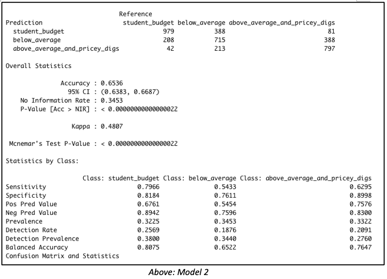
Consider both models below which were each created with 3811 rows of data representing 60% of the total dataset. Both models were created with the same predictor variables, such as the number of bedrooms, bathrooms, property type, location, etc. But in Model 1, the data was binned into 4 equal groups while in Model 2, the data was binned into 3 equal groups. The model summary for Model 1 showed the model has an accuracy of 54.19%, which is good considering that this performance is slightly more than double the No Information Rate (Naïve Rate). Model 2’s accuracy’s level is at 65.36%, a level which is nearly double its No Information Rate.

These are encouraging results but in our Airbnb example, we are more interested in knowing how well our model performs when it is asked to classify properties into any of the classes used in the model. For this reason, it is worth considering the true positive rate i.e. ‘sensitivity’. Model 1 is better at predicting the true positives (‘sensitivity’) for classes at opposite ends of the spectrum. This suggests Model 1 has difficulty reading nuances. On the other hand, Model 2’s performance in this regard is comparatively more balanced.
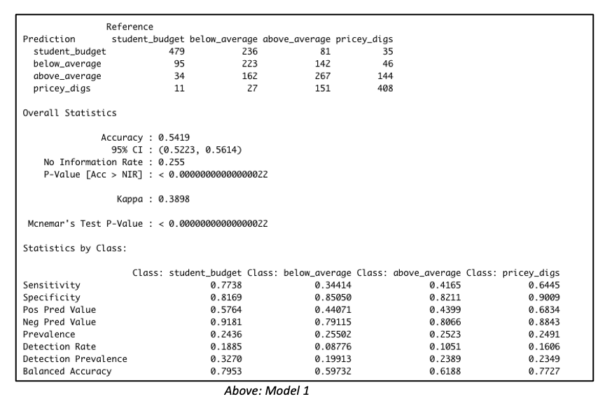
Naive Bayes model with four classification outcome


Naive Bayes output with three classification outcome


But wait – let’s get back to our original goal.  While overall accuracy is good to see, what we are most interested in here is identifying that high-end price group.  Owners of such units will be the best targets for our all-in-one concierge service.  Therefore, let’s dive a bit deeper to examine this model’s suitability for identifying such properties. 

By running the predict() function with the type=’raw’ parameter included, we can view the associated probabilities for each outcome class, and then rank records by probability of belonging to some particular outcome group. 

Taking this approach with the validation set, we find that among the 100 records identified by the model as most likely to land in the top tier group, 96 truly belonged to “Above Average and Pricey Digs.”   Among the 150 likeliest, 140 units, or 93.33%, actually belonged to that group, and among the 200 likeliest, 185 units, or 92.5%, were truly in that top tier. 

But that’s not all. It is worth going one step further by evaluating the model with lift charts or decile-wise lift charts because these charts determine how effectively our model ‘skims the cream’.

The decile-wise lift charts below illustrate how effectively the model can predict membership in the ‘above average and pricey digs’ group. When the model is used to classify the top 27% properties in this category, its performance is more than 3.5x better than a random guess.
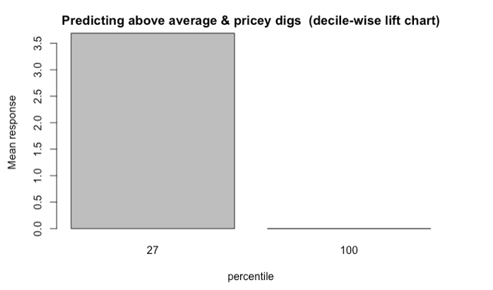
Decile-wise lift chart shows the model is 3.5 times better at classifying the top 27 percent properties

Another way to assess the model’s ability to identify top-tier rentals is with a two-dimensional lift chart.  Such a chart only works with two-outcome class scenarios, so we start here by collapsing the first and second tiers together, and then labelling that group as “other.”  
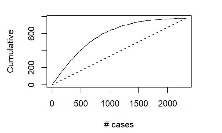
Gains chart shows among the 500 records that the model says are most likely to land in the Above Average & Pricey Digs Tier, just over 400 truly did belong to that group

In the entire validation set, there are 780 units that land in the highest price tier.  The values along the x-axis represent all the validation set records, ranked in order of their probability of belonging to the highest-tier class.  The y-axis shows the number of correct predictions.  The solid line represents the model’s performance – it shows us, for instance, that among the 500 records that the model says are most likely to land in the Above Average & Pricey Digs Tier, just over 400 truly did belong to that group.  The line flattens out at around x=1500, because by that point, the model has already identified nearly all of the records that truly belonged to this outcome class. 

The dotted line, by contrast, shows how effective a model would be if it simply labelled all the records as belonging to the top tier.  Since 33.6%, of the validation records belong to this group, each x-axis value here corresponds to a y-axis value that is exactly 33.6% as large.  The difference between the solid line and the dotted line represents the model’s improvement as the number of cases increases.

What do these results mean for the concierge service?  Let’s revisit our original assumptions: 


  • such a service would most likely appeal to the owners of properties in the highest pricing tier;
  • the initial outreach efforts should be made to owners of properties not already registered with Airbnb; and that
  • the new service has a limited budget, and therefore needs to carefully focus its outreach efforts only on that tier of properties whose owners would be likeliest to use it
Given these assumptions, our primary interest does not lie with overall model accuracy.  The model’s ability to distinguish between the bottom two pricing tiers is almost immaterial to us; however, we are keenly interested in the answer to this question:  When the model predicts that a property will belong to the highest pricing tier, how often is it correct? 

As demonstrated here, the model delivers quite effectively in this regard, especially when we maintain a relatively narrow focus on the properties that are most likely to be top tier.  Splashy magazine inserts, Super Bowl advertisements, and big-ticket endorsements from celebrities might be in the cards for this service down the road, after it spreads across the globe and prepares for its IPO roadshow.  For now, though, the hyper-specific focus that can come from “skimming the cream” off the top of those Naïve Bayes model probability predictions may be the surest next step for this service’s success. 

Data source: Inside Airbnb
 

Azure Machine Learning For R Practitioners With The R SDK

[This article was first published on the Azure Medium channel, and kindly contributed to R-bloggers]. (You can report issue about the content on this page here)


As probably you already know, Microsoft provided its Azure Machine Learning SDK for Python to build and run machine learning workflows, helping organizations to use massive data sets and bring all the benefits of the Azure cloud to machine learning.

Although Microsoft initially invested in R as the Advanced Analytics preferred language introducing the SQL Server R server and R services in the 2016 version, they abruptly shifted their attention to Python, investing exclusively on it. This basically happened for the following reasons:

  • Python’s simple syntax and readability make the language accessible to non-programmers
  • The most popular machine learning and deep learning open source libraries (such as Pandas, scikit-learn, TensorFlow, PyTorch, etc.) are deeply used by the Python community
  • Python is a better choice for productionalization: it’s relatively very fast; it implements OOPs concepts in a better way; it is scalable (Hadoop/Spark); it has better functionality to interact with other systems; etc.

Azure ML Python SDK Main Key Points

One of the most valuable aspects of the Python SDK is its ease to use and flexibility. You can simply use just few classes, injecting them into your existing code or simply referring to your script files into method calls, in order to accomplish the following tasks:

  • Explore your datasets and manage their lifecycle
  • Keep track of what’s going on into your machine learning experiments using the Python SDK tracking and logging features
  • Transform your data or train your models locally or using the best cloud computation resources needed by your workloads
  • Register your trained models on the cloud, package them into container image and deploy them on web services hosted in Azure Container Instances or Azure Kubernetes Services
  • Use Pipelines to automate workflows of machine learning tasks (data transformation, training, batch scoring, etc.)
  • Use automated machine learning (AutoML) to iterate over many combinations of defined data transformation pipelines, machine learning algorithms and hyperparameter settings. It then finds the best-fit model based on your chosen performance metric.

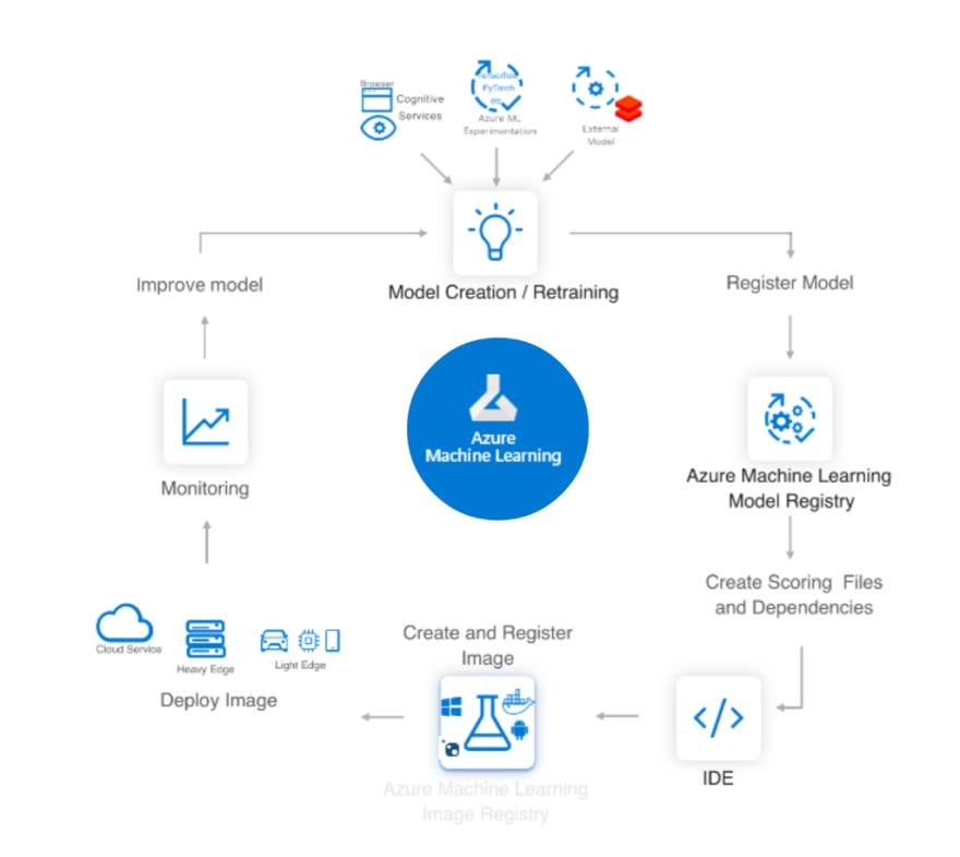
In summary, the scenario is the following one:

AI/ML lifecycle using Azure ML
fig. 1 — AI/ML lifecycle using Azure ML

What About The R Community Engagement?

In the last 3 years Microsoft pushed a lot over the Azure ML Python SDK, making it a stable product and a first class citizen of the Azure cloud. But they seem to have forgotten all the R professionals who developed a huge amount of data science project all around the world.

We must not forget that in Analytics and Data Science the key of success of a project is to quickly try out a large number of analytical tools and find what’s the best one for the case in analysis. R was born for this reason. It has a lot of flexibility when you want to work with data and build some model, because it has tons of packages and easy of use visualization functionality. That’s why a lot of Analytics projects are developed using R by many statisticians and data scientists.

Fortunately in the last months Microsoft extended a hand to the R community, releasing a new project called Azure Machine Learning R SDK.

Can I Use R To Spin The Azure ML Wheels?

Starting from October 2019 Microsoft released a R interface for Azure Machine Learning SDK on GitHub. The idea behind this project is really straightforward. The Azure ML Python SDK is a way to simplify the access and the use of the Azure cloud storage and computation for machine learning purposes keeping the main code as the one a data scientist developed on its laptop.

Why not allow the Azure ML infrastructure to run also R code (using proper “cooked” Docker images) and let R data scientists call the Azure ML Python SDK methods using R functions?

The interoperability between Python and R is obtained thanks to reticulate. So, once the Python SDK module azureml is imported into any R environment using the import function, functions and other data within the azureml module can be accessed via the $ operator, like an R list.

Obviously, the machine hosting your R environment must have Python installed too in order to make the R SDK work properly.

Let’s start to configure your preferred environment.

Set Up A Development Environment For The R SDK

There are two option to start developing with the R SDK:

  1. Using an Azure ML Compute Instance (the fastest way, but not the cheaper one!)
  2. Using your machine (laptop, VM, etc.)

Set Up An Azure ML Compute Instance

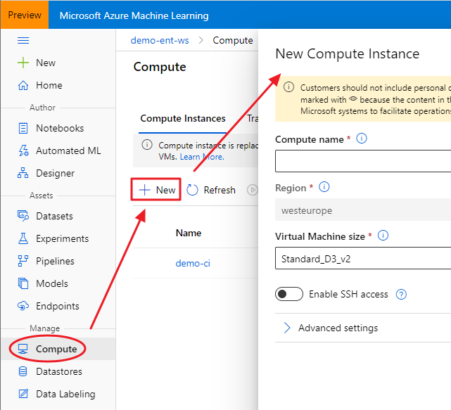
Once you created an Azure Machine Learning Workspace through the Azure portal (a basic edition is enough), you can access to the brand new Azure Machine Learning Studio. Under the Compute section, you can create a new Compute Instance, choosing its name and its sizing:

Create an Azure ML Compute Instance
fig. 2 — Create an Azure ML Compute Instance

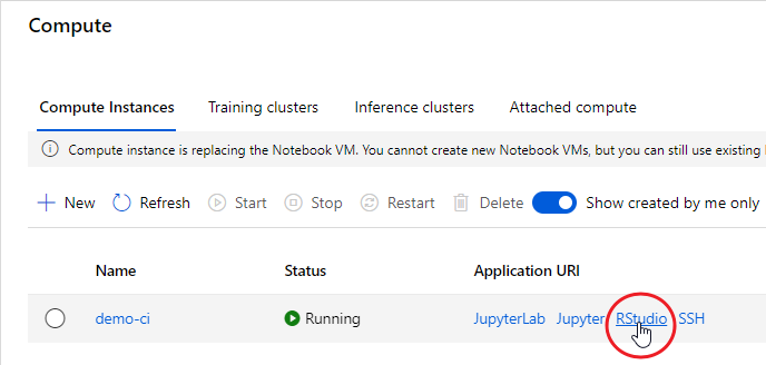
The advantage of using a Compute Instance is that the most used software and libraries by data scientists are already installed, including the Azure ML Python SDK and RStudio Server Open Source Edition. That said, once your Compute Instance is started, you can connect to RStudio using the proper link:

Launch RStudio from a started Compute Intstance
fig. 3 — Launch RStudio from a started Compute Intstance

At the end of your experimentation, remember to shut down your Compute Instance, otherwise you’ll be charged according to the chosen plan:

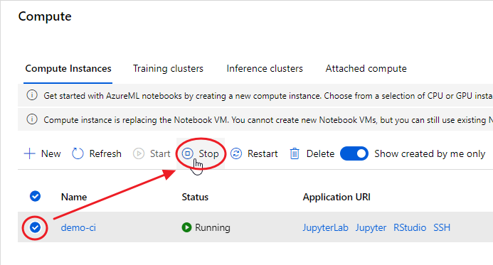
Remember to shut down your Compute Instance
fig. 4 — Remember to shut down your Compute Instance

Set Up Your Machine From Scratch

First of all you need to install the R engine from CRAN or MRAN. Then you could also install RStudio Desktop, the preferred IDE of R professionals.

The next step is to install Conda, because the R SDK needs to bind to the Python SDK through reticulate. If you really don’t need Anaconda for specific purposes, it’s recommended to install a lightweight version of it, Miniconda. During its installation, let the installer add the conda installation of Python to your PATH environment variable.

Install The R SDK

Open your RStudio, simply create a new R script (File → New File → R Script) and install the last stable version of Azure ML R SDK package (azuremlsdk) available on CRAN in the following way:

install.packages("remotes")
remotes::install_cran("azuremlsdk")


If you want to install the latest committed version of the package from GitHub (maybe because the product team has fixed an annoying bug), you can instead use the following function:
remotes::install_github('https://github.com/Azure/azureml-sdk-for-r')

During the installation you could get this error:

Timezone error
fig. 5 — Timezone error

In this case, you just need to set the TZ environment variable with your preferred timezone:

Sys.setenv(TZ="GMT")

Then simply re-install the R SDK.

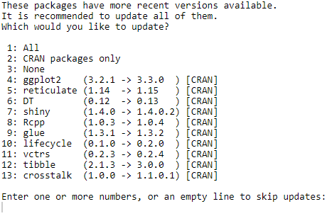
You may also be asked to update some dependent packages:

Dependent packages to be updated
fig. 6 — Dependent packages to be updated

If you don’t have any requirement about dependencies in your project, it’s always better to update them all (put focus on the prompt in the console; press 1; press enter).

If you are on your Compute Instance and you get a warning like the following one:

Warning about non-system installation of Python
fig. 7 — Warning about non-system installation of Python

just put the focus on the console and press “n”, since the Compute Instance environment already has a Conda installation. Microsoft engineers are already investigating on this issue.

You need then to install the Azure ML Python SDK, otherwise your azuremlsdk R package won’t work. You can do that directly from RStudio thanks to an azuremlsdk function:

azuremlsdk::install_azureml(remove_existing_env = TRUE)

The remove_existing_env parameter set to TRUE will remove the default Azure ML SDK environment r-reticulate if previously installed (it’s a way to clean up a Python SDK installation).

Just keep in mind that in this way you’ll install the version of the Azure ML Python SDK expected by your installed version of the azuremlsdk package. You can check what version you will install putting the cursor over the install_azureml function and visualizing the code definition clicking F2:

install_azureml code definition
fig. 8 — install_azureml code definition

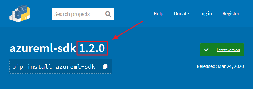
Sometimes there are new feature and fixes on the latest version of the Python SDK. If you need to install it, first check what version is available on this link:

Azure ML Python SDK latest version
fig. 9 — Azure ML Python SDK latest version

Then use that version number in the following code:

azuremlsdk::install_azureml(version = "1.2.0", remove_existing_env = TRUE)

Sometimes you may need to install an updated version of a single component of the Azure ML Python SDK to test, for example new features. Supposing you want to update the Azure ML Data Prep SDK, here the code you could use:

reticulate::py_install("azureml-dataprep==1.4.2", envname = "r-reticulate", pip = TRUE)

In order to check if the installation is working correctly, try this:

library(azuremlsdk)
get_current_run()

It should return something like this:

Checking that azuremlsdk is correctly installed
fig. 10 — Checking that azuremlsdk is correctly installed

Great! You’re now ready to spin the Azure ML wheels using your preferred programming language: R!


Conclusions

After a long period during which Microsoft focused exclusively on Python SDK to enable data scientists to benefit from Azure computing and storage services, they recently released the R SDK too. This article focuses on the steps needed to install the Azure Machine Learning R SDK on your preferred environment.

Next articles will deal with the R SDK main capabilities.

R as learning tool: solving integrals


Integrals are so easy only math teachers could make them difficult.When I was in high school I really disliked math and, with hindsight, I would say it was just because of the the prehistoric teaching tools (when I saw this video I thought I’m not alone). I strongly believe that interaction CAUSES learning (I’m using “causes” here on purpose being quite aware of the difference between correlation and causation), practice should come before theory and imagination is not a skill you, as a teacher, could assume in your students. Here follows a short and simple practical explanation of integrals. The only math-thing I will write here is the following: f(x) = x + 7. From now on everything will be coded in R. So, first of all, what is a function? Instead of using the complex math philosophy let’s just look at it with a programming eye: it is a tool that takes something in input and returns something else as output. For example, if we use the previous tool with 2 as an input we get a 9. Easy peasy. Let’s look at the code:
# here we create the tool (called "f")
# it just takes some inputs and add it to 7
f <- function(x){x+7}

# if we apply it to 2 it returns a 9
f(2)
9

Then the second question comes by itself. What is an integral? Even simpler, it is just the sum of this tool applied to many inputs in a range. Quite complicated, let’s make it simpler with code: 
# first we create the range of inputs
# basically x values go from 4 to 6 
# with a very very small step (0.01)
# seq stands for sequence(start, end, step)


x <- seq(4, 6, 0.01) 
x
4.00 4.01 4.02 4.03 4.04 4.05 4.06 4.07...

x[1]
4

x[2]
4.01
As you see, x has many values and each of them is indexed so it’s easy to find, e.g. the first element is 4 (x[1]). Now that we have many x values (201) within the interval from 4 to 6, we compute the integral.
# since we said that the integral is 
# just a sum, let's call it IntSum and 
# set it to the start value of 0
# in this way it will work as an accumulator
IntSum = 0
Differently from the theory in which the calculation of the integral produces a new non-sense formula (just kidding, but this seems to be what math teachers are supposed to explain), the integral does produce an output, i.e. a number. We find this number by summing the output of each input value we get from the tool (e.g. 4+7, 4.01+7, 4.02+7, etc) multiplied by the step between one value and the following (e.g. 4.01-4, 4.02-4.01, 4.03-4.02, etc). Let’s clarify this, look down here:
# for each value of x 
for(i in 2:201){
    
    # we do a very simple thing:
    # we cumulate with a sum
    # the output value of the function f 
    # multiplied by each steps difference
    
    IntSum = IntSum + f(x[i])*(x[i]-x[i-1])
    
    
    # So for example,  
    # with the first and second x values the numbers will be:
    #0.1101 = 0 + (4.01 + 7)*(4.01 - 4)
    
    # with the second and third:
    #0.2203 = 0.1101 + (4.02 + 7)*(4.02 - 4.01)
    
    # with the third and fourth:
    #0.3306 = 0.2203 + (4.03 + 7)*(4.03 - 4.02)
    
    # and so on... with the sum (integral) growing and growing
    # up until the last value
}

IntSum
24.01
Done! We have the integral but let’s have a look to the visualization of this because it can be represented and made crystal clear. Let’s add a short line of code to serve the purpose of saving the single number added to the sum each time. The reason why we decide to call it “bin” instead of, for example, “many_sum” will be clear in a moment.
# we need to store 201 calculation and we
# simply do what we did for IntSum but 201 times
bin = rep(0, 201)
bin
0 0 0 0 0 0 0 0 0 0 0 0 ...
Basically, we created a sort of memory to host each of the calculation as you see down here:
for (i in 2:201){
    
    # the sum as earlier
    IntSum = IntSum + f(x[i])*(x[i]-x[i-1])
    
    # overwrite each zero with each number
    bin[i] = f(x[i])*(x[i]-x[i-1])
}

IntSum
24.01

bin
0.0000 0.1101 0.1102 0.1103 0.1104 0.1105 ..

sum(bin)
24.01
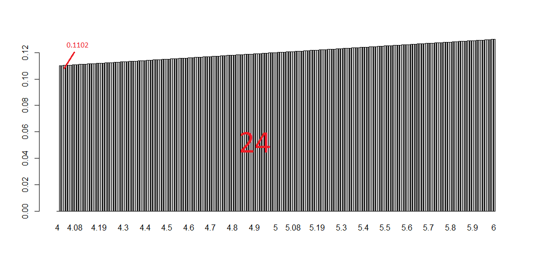
Now if you look at the plot below you get the whole story: each bin is a tiny bar with a very small area and is the smallest part of the integral (i.e. the sum of all the bins).
# plotting them all
barplot(bin, names.arg=x)
This tells you a lot about the purpose of integral and the possibility of calculating areas of curvy surfaces. To have an idea of this just change the function f with, let’s say, sin(x) or log(x). What is happening? And what if you increase/decrease the number of bins? Have fun replicating the code changing some numbers and functions. Integrals should be clearer in the end. That’s all folks! #R #rstats #maRche #Rbloggers 

“Print hello”​ is not enough. A collection of Hello world functions.


I guess I wrote my R “hello world!” function 7 or 8 years ago while approaching R for the first time. And it is too little to illustrate the basic syntax of a programming language for a working program to a wannabe R programmer. Thus, here follows a collection of basic functions that may help a bit more than the famed piece of code.

######################################################
############### Hello world functions ################
######################################################
##################################
# General info
fun <- function( arguments ) { body }


##################################
foo.add <- function(x,y){
  x+y
}

foo.add(7, 5)

----------------------------------

foo.above <- function(x){
  x[x>10]
}

foo.above(1:100)

----------------------------------

foo.above_n <- function(x,n){
  x[x>n]
}

foo.above_n(1:20, 12)

----------------------------------

foo = seq(1, 100, by=2)
foo.squared = NULL

for (i in 1:50 ) {
  foo.squared[i] = foo[i]^2
}

foo.squared

----------------------------------

a <- c(1,6,7,8,8,9,2)

s <- 0
for (i in 1:length(a)){
  s <- s + a[[i]]
}
s

----------------------------------

a <- c(1,6,7,8,8,9,2,100)

s <- 0
i <- 1
while (i <= length(a)){
  s <- s + a[[i]]
  i <- i+1
}
s

----------------------------------

FunSum <- function(a){
  s <- 0
  i <- 1
  while (i <= length(a)){
    s <- s + a[[i]]
    i <- i+1
  }
  print(s)
}

FunSum(a)

-----------------------------------

SumInt <- function(n){
  s <- 0
  for (i in 1:n){
    s <- s + i
  }
  print(s)  
}

SumInt(14)

-----------------------------------
# find the maximum
# right to left assignment
x <- c(3, 9, 7, 2)

# trick: it is necessary to use a temporary variable to allow the comparison by pairs of
# each number of the sequence, i.e. the process of comparison is incremental: each time
# a bigger number compared to the previous in the sequence is found, it is assigned as the
# temporary maximum
# Since the process has to start somewhere, the first (temporary) maximum is assigned to be
# the first number of the sequence

max <- x[1]
for(i in x){
  tmpmax = i
  if(tmpmax > max){
    max = tmpmax
  }
}

max

x <- c(-20, -14, 6, 2)
x <- c(-2, -24, -14, -7)

min <- x[1]
for(i in x){
  tmpmin = i
  if(tmpmin < min){
    min = tmpmin
  }
}

min

----------------------------------
# n is the nth Fibonacci number
# temp is the temporary variable

Fibonacci <- function(n){
  a <- 0
  b <- 1
  for(i in 1:n){
    temp <- b
    b <- a
    a <- a + temp
  }
  return(a)
}

Fibonacci(13)

----------------------------------
# R available factorial function
factorial(5)

# recursive function: ff
ff <- function(x) {
  if(x<=0) {
    return(1)
  } else {
    return(x*ff(x-1)) # function uses the fact it knows its own name to call itself
  }
}
ff(5)

----------------------------------

say_hello_to <- function(name){
  paste("Hello", name)
} 
say_hello_to("Roberto")

----------------------------------

foo.colmean <- function(y){
  nc <- ncol(y)
  means <- numeric(nc)
  for(i in 1:nc){
    means[i] <- mean(y[,i])
  }
  means
}

foo.colmean(airquality)

----------------------------------

foo.colmean <- function(y, removeNA=FALSE){
  nc <- ncol(y)
  means <- numeric(nc)
  for(i in 1:nc){
    means[i] <- mean(y[,i], na.rm=removeNA)
  }
  means
}

foo.colmean(airquality, TRUE)

----------------------------------

foo.contingency <- function(x,y){
  nc <- ncol(x)
  out <- list() 
  for (i in 1:nc){
    out[[i]] <- table(y, x[,i]) 
  }
  names(out) <- names(x)
  out
}

set.seed(123)
v1 <- sample(c(rep("a", 5), rep("b", 15), rep("c", 20)))
v2 <- sample(c(rep("d", 15), rep("e", 20), rep("f", 5)))
v3 <- sample(c(rep("g", 10), rep("h", 10), rep("k", 20)))

data <- data.frame(v1, v2, v3)

foo.contingency(data,v3)
That's all folks! #R #rstats #maRche #Rbloggers This post is also shared in LinkedIn and www.r-bloggers.com

Web data acquisition: from database to dataframe for data analysis and visualization (Part 4)

The previous post described how the deeply nested JSON data on fligths were parsed and stored in an R-friendly database structure. However, looking into the data, the information is not yet ready for statistical analysis and visualization and some further processing is necessary before extracting insights and producing nice plots. In the parsed batch, it is clearly visible the redundant structure of the data with the flight id repeted for each segment of each flight. This is also confirmed with the following simple check as the rows of the dataframe are more than the unique counts of the elements in the id column.
dim(data_items)
[1] 397  15

length(unique(data_items$id))
201

# real time changes of data could produce different results
This implies that the information of each segment of each flight has to be aggregated and merged in a dataset as single observations of a statistical analysis between, for example, price and distance. First, a unique primary key for each observation has to be used as reference variable to uniquely identify each element of the dataset.
library(plyr) # sql like functions
library(readr) # parse numbers from strings
 
data_items <- data.frame(data_items)
 
# id (primary key)
data <- data.frame(unique(data_items$id))
colnames(data) <- c('id')
 
# n° of segment
n_segment <- aggregate(data_items['segment.id'], by=data_items['id'], length)
data <- join(data, n_segment, by='id', type='left', match='first') # sql left join
# mileage
mileage <- aggregate(data_items['segment.leg.mileage'], by=data_items['id'], sum)
data <- join(data, mileage, by='id', type='left', match='first') # sql left join
# price
price <- data.frame('id'=data_items$id, 'price'=parse_number(data_items$saleTotal))
data <- join(data, price, by='id', type='left', match='first') # sql left join
# dataframe
colnames(data) <- c('id','segment', 'mileage', 'price')
head(data)

The aggregation of mileage and price using the unique primary key allows to set up a dataframe ready for statistical analysis and data visualization. Current data tells us that there is a maximum of three segments in the connection between FCO and LHR with a minimum price of around EUR 122 and a median around EUR 600.

# descriptive statistics
summary(data)
 
 
# histogram price & distance
g1 <- ggplot(data, aes(x=price)) + 
  geom_histogram(bins = 50) +  
  ylab("Distribution of the Price (EUR)") +
  xlab("Price (EUR)") 
 
g2 <- ggplot(data, aes(x=mileage)) + 
  geom_histogram(bins = 50) +  
  ylab("Distribution of the Distance") +
  xlab("Distance (miles)")
 
grid.arrange(g1, g2)
# price - distance relationship
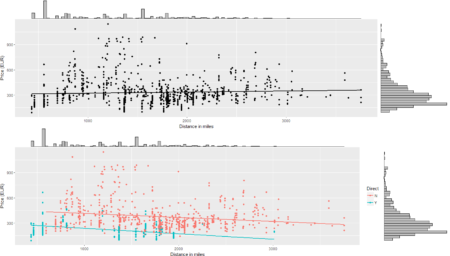
s0 <- ggplot(data = data, aes(x = mileage, y = price)) +
    geom_smooth(method = "lm", se=FALSE, color="black") +
    geom_point() + labs(x = "Distance in miles", y = "Price (EUR)")
s0 <- ggMarginal(s0, type = "histogram", binwidth = 30)
s0

Of course, plenty of other analysis and graphical representations using flights features are possible given the large set of variables available in QPX Express API and the availability of data in real time.
To conclude the 4-step (flight) trip from data acquisition to data analysis, let's recap the most important concepts described in each of the post: 1) Client-Server connection 2) POST request in R 3) Data parsing and structuring 4) Data analysis and visualization
That's all folks! #R #rstats #maRche #json #curl #qpxexpress #Rbloggers This post is also shared in www.r-bloggers.com