Batched Imputation for High Dimensional Missing Data Problems

Interested in publishing a one-time post on R-bloggers.com? Press here to learn how.

---

High dimensional data spaces are notoriously associated with slower computation time, whether imputation or some other operation. As such, in high dimensional contexts many imputation methods run out of gas, and fail to converge (e.g., MICE, PCA, etc., depending on the size of the data). Further, though some approaches to high dimensional imputation exist, most are limited by being unable to simultaneously and natively handle mixed-type data.

To address these problems of either inefficient or slow computation time, as well as the complexities associated with mixed-type data, I recently released the first version of a new algorithm, hdImpute,  for fast, accurate imputation for high dimensional missing data problems. The algorithm is built on top of missForest and missRanger, with chained random forests as the imputation engine.

The benefit of the hdImpute is in simplifying the computational burden via a batch process comprised of a few stages. First, the algorithm divides the data space into smaller subsets of data based on cross-feature correlations (i.e., column-wise instead of row-wise subsets). The algorithm then imputes each batch, the size of which is controlled by a hyperparameter, batch, set by the user. Then, the algorithm continues to subsequent batches until all batches are individually imputed. Then, the final step joins the completed, imputed subsets and returns a single, completed data frame. 

Let’s walk through a brief demo with some simulated data. First, create the data.

# load a couple libraries
library(tidyverse)
library(hdImpute) # using v0.1.0 here

# create the data
{
set.seed(1234)

data <- data.frame(X1 = c(1:6),
X2 = c(rep("A", 3), 
rep("B", 3)), 
X3 = c(3:8),
X4 = c(5:10),
X5 = c(rep("A", 3), 
rep("B", 3)), 
X6 = c(6,3,9,4,4,6))

data <- data[rep(1:nrow(data), 500), ] # expand/duplicate rows

data <- data[sample(1:nrow(data)), ] # shuffle rows
}

Next, take a look to make sure we are indeed working with mixed-type data. 

# quick check to make sure we have mixed-type data
data %>% 
map(., class) %>% 
unique()

> [[1]] [1] "integer" [[2]] [1] "character" [[3]] [1] "numeric"

Good to go: three data classes represented in our data object. Practically, the value of this feature is that there is no requirement for lengthy preprocessing of the data, unless desired by the user of course.

Finally, introduce some NA’s to our data object, and store in d.

# produce NAs (30%)
d <- missForest::prodNA(data, noNA = 0.30) %>% 
as_tibble()

Importantly, the package allows for two approaches to use hdImpute: in stages (to allow for more flexibility, or, e.g., tying different stages into different points of a modeling pipeline); or as a single call to hdImpute(). Let’s take a look at the first approach via stages. 

Approach 1: Stages

To use hdImpute in stages, three functions are used, which comprise each of the stages of the algorithm: 

1. feature_cor(): creates the correlation matrix. Note: Dependent on the size and dimensionality of the data as well as the speed of the machine, this preprocessing step could take some time. 

2. flatten_mat(): flattens the correlation matrix from the previous stage, and ranks the features based on absolute correlations. The input for flatten_mat() should be the stored output from feature_cor().

3. impute_batches(): creates batches based on the feature rankings from flatten_mat(), and then imputes missing values for each batch, until all batches are completed. Then, joins the batches to give a completed, imputed data set.
   
   Here’s the full workflow.

# stage 1: calculate correlation matrix and store as matrix/array
all_cor <- feature_cor(d)

# stage 2: flatten and rank the features by absolute correlation and store as df/tbl
flat_mat <- flatten_mat(all_cor) # can set return_mat = TRUE to print the flattened and ranked feature list

# stage 3: impute, join, and return
imputed1 <- impute_batches(data = d,
features = flat_mat, 
batch = 2)

# take a look at the completed data
imputed1

d # compare to the original if desired

Of note, setting return_mat = TRUE returns all cross-feature correlations as previously mentioned. But calling the stored object (regardless of the value passed to return_mat) will return the vector of ranked features based on absolute correlation from calling flatten_mat(). Thus, the default for return_mat is set to FALSE, as it isn’t necessary to inspect the cross-feature correlations, though users certainly can. But all that is required for imputation in stage 3 is the vector of ranked features (passed to the argument features), which will be split into batches based on their position in the ranked vector.

That’s it! We have a completed data frame returned via hdImpute. The speed and accuracy of the algorithm are better understood in larger scale benchmarking experiments. But I hope the logic is clear enough from this simple demonstration. 

Approach 2: Single Call

Finally, consider the simpler, yet less flexible approach of making a single call to hdImpute(). There are only two required arguments: data (original data with missing values) and batch (number of batches to create from the data object). Here’s what this approach might look like using our simulated data from before:

# fit and store in imputed2
imputed2 <- hdImpute(data = d, batch = 2)

# take a look
imputed2

# make sure you get the same results compared to the stages approach above
imputed1 == imputed2

Visually Comparing

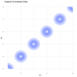
Though several methods and packages exist to explore imputation error, a quick approach to comparing error between the imputed values and the original (complete) data is to visualize the contour of the relationship between a handful of features. For example, take a look at the contour plot of the original data.

data %>%
select(X1:X3) %>% 
ggplot(aes(x = X1, y = X3, fill = X2)) + 
geom_density_2d() + 
theme_minimal() + 
labs(title = "Original (Complete) Data")

Next, here’s the same plot but for the imputed set. 

imputed2 %>% 
select(X1:X3) %>% 
ggplot(aes(x = X1, y = X3, fill = X2)) + 
geom_density_2d() + 
theme_minimal(). + 
labs(title = "Imputed (Complete) Data")

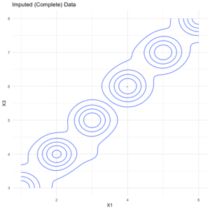
As expected, the imputed version has a bit of error (looser distributions) relative to the original version. But the overall pattern is quite similar, suggesting hdImpute did a fair job of imputing plausible values.

Contribute

To dig more into the package, check out the repo, which includes source code, a getting started vignette, tests, and all other documentation.

As the software is in its infancy, contribution at any level is welcomed, from bug reports to feature suggestions. Feel free to open an issue or PR to request the change or contribute. 

Thanks and I hope this helps ease high dimensional imputation!