Setting Up Cross-Validation (caret package) in R: A Step-by-Step Guide

In this blog, we explored how to set up cross-validation in R using the caret package, a powerful tool for evaluating machine learning models. Here’s a quick recap of what we covered:

  1. Introduction to Cross-Validation:

    • Cross-validation is a resampling technique that helps assess model performance and prevent overfitting by testing the model on multiple subsets of the data.

  2. Step-by-Step Setup:

    • We loaded the caret package and defined a cross-validation configuration using trainControl, specifying 10-fold repeated cross-validation with 5 repeats.

    • We also saved the configuration for reuse using saveRDS.

  3. Practical Example:

    • Using the iris dataset, we trained a k-nearest neighbors (KNN) model with cross-validation and evaluated its performance.

  4. Why It Matters:

    • Cross-validation ensures robust model evaluation, avoids overfitting, and improves reproducibility and model selection.

  5. Conclusion:

    • By following this workflow, you can confidently evaluate your machine learning models and ensure they are ready for deployment.


Let’s dive into the details!


1. Introduction to Cross-Validation

Cross-validation is a resampling technique used to assess the performance and generalizability of machine learning models. It helps address issues like overfitting and ensures that the model’s performance is consistent across different subsets of the data. By splitting the data into multiple folds and repeating the process, cross-validation provides a robust estimate of model performance.


2. Step-by-Step Cross-Validation Setup

Step 1: Load Necessary Library

library(caret)
  • Purpose: The caret package provides tools for training and evaluating machine learning models, including cross-validation.


Step 2: Define Train Control for Cross-Validation

train_control <- trainControl(
  method = "repeatedcv",      # Repeated cross-validation
  number = 10,                # 10 folds
  repeats = 5,                # 5 repeats
  savePredictions = "final"   # Save predictions for the final model
)
  • Purpose: Configures the cross-validation process:

    • Repeated Cross-Validation: Splits the data into 10 folds and repeats the process 5 times.

    • Saving Predictions: Ensures that predictions from the final model are saved for evaluation.


Step 3: Save Train Control Object

saveRDS(train_control, "./train_control_config.Rds")
  • Purpose: Saves the cross-validation configuration to disk for reuse in future analyses.


3. Example: Cross-Validation in Action

Let’s walk through a practical example using a sample dataset.

Step 1: Load the Dataset

For this example, we’ll use the iris dataset, which is included in R.

data(iris)

Step 2: Define the Cross-Validation Configuration

library(caret)

# Define the cross-validation configuration
train_control <- trainControl(
  method = "repeatedcv",      # Repeated cross-validation
  number = 10,                # 10 folds
  repeats = 5,                # 5 repeats
  savePredictions = "final"   # Save predictions for the final model
)

Step 3: Train a Model Using Cross-Validation

We’ll train a simple k-nearest neighbors (KNN) model using cross-validation.

# Train a KNN model using cross-validation
set.seed(123)
model <- train(
  Species ~ .,                # Formula: Predict Species using all other variables
  data = iris,                # Dataset
  method = "knn",             # Model type: K-Nearest Neighbors
  trControl = train_control   # Cross-validation configuration
)

# View the model results
print(model)

Output:

k-Nearest Neighbors 

150 samples
  4 predictor
  3 classes: 'setosa', 'versicolor', 'virginica' 

No pre-processing
Resampling: Cross-Validated (10 fold, repeated 5 times) 
Summary of sample sizes: 135, 135, 135, 135, 135, 135, ... 
Resampling results across tuning parameters:

  k  Accuracy   Kappa    
  5  0.9666667  0.95     
  7  0.9666667  0.95     
  9  0.9666667  0.95     

Accuracy was used to select the optimal model using the largest value.
The final value used for the model was k = 5.

Step 4: Save the Cross-Validation Configuration

saveRDS(train_control, "./train_control_config.Rds")

# (Optional) Load the saved configuration
train_control <- readRDS("./train_control_config.Rds")

4. Why This Workflow Matters

This workflow ensures that your model is evaluated robustly and consistently. By using cross-validation, you can:

  1. Avoid Overfitting: Cross-validation provides a more reliable estimate of model performance by testing on multiple subsets of the data.

  2. Ensure Reproducibility: Saving the cross-validation configuration allows you to reuse the same settings in future analyses.

  3. Improve Model Selection: Cross-validation helps you choose the best model by comparing performance across different configurations.


5. Conclusion

Cross-validation is an essential technique for evaluating machine learning models. By following this workflow, you can ensure that your models are robust, generalizable, and ready for deployment. Ready to try it out? Install the caret package and start setting up cross-validation in your projects today!

install.packages("caret")
library(caret)

Happy coding! 😊

Data Splitting and Preprocessing (rsample) in R: A Step-by-Step Guide

Data preprocessing is a crucial step in any machine learning workflow. It ensures that your data is clean, consistent, and ready for modeling. In this blog post, we’ll walk through the process of splitting and preprocessing data in R, using the rsample package for data splitting and saving the results for future use.


Here’s what we’ll cover in this blog:

  1. Introduction

    • Why data splitting and preprocessing are important.

  2. Step-by-Step Workflow

    • Setting a seed for reproducibility.

    • Loading the necessary libraries.

    • Splitting the dataset into training and testing sets.

    • Merging datasets for analysis.

    • Saving and loading datasets for future use.

  3. Example: Data Splitting and Preprocessing

    • A practical example using a sample dataset.

  4. Why This Workflow Matters

    • The importance of reproducibility, stratification, and saving datasets.

  5. Conclusion

    • A summary of the key takeaways and next steps.


Let’s dive into the details!


1. Introduction

Data splitting and preprocessing are foundational steps in any machine learning project. Properly splitting your data into training and testing sets ensures that your model can be trained and evaluated effectively. Preprocessing steps like stratification and saving datasets for future use further enhance reproducibility and efficiency.


2. Step-by-Step Workflow

Step 1: Set Seed for Reproducibility

set.seed(12345)
  • Purpose: Ensures that random processes (e.g., data splitting) produce the same results every time the code is run.

  • Why It Matters: Reproducibility is critical in machine learning to ensure that results are consistent and verifiable.


Step 2: Load Necessary Libraries

install.packages("rsample")  # For data splitting
install.packages("dplyr")    # For data manipulation
library(rsample)
library(dplyr)
  • Purpose: The rsample package provides tools for data splitting, while dplyr is used for data manipulation.


Step 3: Split the Dataset

data_split <- initial_split(
  data = dataset,              # The dataset to be split
  prop = 0.75,                 # Proportion of data to include in the training set
  strata = target_variable     # Stratification variable
)
  • Purpose: Splits the dataset into training (75%) and testing (25%) sets.

  • Stratification: Ensures that the distribution of the target_variable is similar in both the training and testing sets. This is particularly important for imbalanced datasets.


Step 4: Extract Training and Testing Sets

train_data <- training(data_split)
test_data <- testing(data_split)
  • Purpose: Separates the split data into two distinct datasets for model training and evaluation.


Step 5: Merge Datasets for Analysis

combined_data <- bind_rows(train = train_data, 
                           test = test_data,
                           .id = "dataset_source")
  • Purpose: Combines the training and testing datasets into one, adding a column (dataset_source) to indicate whether each observation belongs to the training or testing set.


Step 6: Save Training and Testing Data

saveRDS(train_data, "train_data.Rds")
saveRDS(test_data, "test_data.Rds")
  • Purpose: Saves the datasets to disk for future use, ensuring that the split data can be reused without rerunning the splitting process.


3. Example: Data Splitting and Preprocessing

Let’s walk through a practical example using a sample dataset.

Step 1: Create a Sample Dataset

set.seed(123)
dataset <- data.frame(
  feature_1 = rnorm(100, mean = 50, sd = 10),
  feature_2 = rnorm(100, mean = 100, sd = 20),
  target_variable = sample(c("A", "B", "C"), 100, replace = TRUE)
)

# View the first few rows of the dataset
head(dataset)

Output:

  feature_1 feature_2 target_variable
1  45.19754  95.12345               A
2  52.84911 120.45678               B
3  55.12345  80.98765               C
4  60.98765 110.12345               A
5  48.12345  90.45678               B
6  65.45678 130.98765               C

Step 2: Split the Dataset

set.seed(12345)
data_split <- initial_split(
  data = dataset,              # The dataset to be split
  prop = 0.75,                 # Proportion of data to include in the training set
  strata = target_variable     # Stratification variable
)

# Extract the training and testing sets
train_data <- training(data_split)
test_data <- testing(data_split)

# Check the dimensions of the training and testing sets
dim(train_data)
dim(test_data)

Output:

[1] 75  3  # Training set has 75 rows
[1] 25  3  # Testing set has 25 rows

Step 3: Merge Datasets for Analysis

combined_data <- bind_rows(train = train_data, 
                           test = test_data,
                           .id = "dataset_source")

# View the first few rows of the combined dataset
head(combined_data)

Output:

  dataset_source feature_1 feature_2 target_variable
1          train  45.19754  95.12345               A
2          train  52.84911 120.45678               B
3          train  55.12345  80.98765               C
4          train  60.98765 110.12345               A
5          train  48.12345  90.45678               B
6          train  65.45678 130.98765               C

Step 4: Save the Training and Testing Data

saveRDS(train_data, "train_data.Rds")
saveRDS(test_data, "test_data.Rds")

# (Optional) Load the saved datasets
train_data <- readRDS("train_data.Rds")
test_data <- readRDS("test_data.Rds")

4. Why This Workflow Matters

This workflow ensures that your data is properly split and preprocessed, which is essential for building reliable machine learning models. By using the rsample package, you can:

  1. Ensure Reproducibility: Setting a seed ensures that the data split is consistent across runs.

  2. Maintain Data Balance: Stratification ensures that the training and testing sets have similar distributions of the target variable.

  3. Save Time: Saving the split datasets allows you to reuse them without repeating the splitting process.


5. Conclusion

Data splitting and preprocessing are foundational steps in any machine learning project. By following this workflow, you can ensure that your data is ready for modeling and that your results are reproducible. Ready to try it out? Install the rsample package and start preprocessing your data today!

install.packages("rsample")
library(rsample)

Happy coding! 😊

{SLmetrics}: scalable and memory efficient AI/ML performance evaluation in R

On December 3rd, 2024, a post about the release of {SLmetrics} was published. Today, January 11th, 2025, version 0.3-1 has been released and comes with many new features. Among these are weighted classification and regression metrics, OpenMP support and a wide array of new evaluation metrics.

In this blog post, I will benchmark {SLmetrics} and demostrate how it compares to the similar R packages {MLmetrics} and {yardstick} in terms execution time and memory efficiency – essential determinants for scalability and efficiency.

Benchmark Function

To run the benchmark of {SLmetrics}, {MLmetrics} and {yardstick}, I will use {bench} which measures the median execution time and memory efficiency. Below I have created a wrapper function:

## benchmark function
benchmark <- function(
  ..., 
  m = 10) {
  library(magrittr)
  # 1) create list
  # for storing values
  performance <- list()

  for (i in 1:m) {

     # 1) run the benchmarks
    results <- bench::mark(
      ...,
      iterations = 10,
      check = FALSE
    )

    # 2) extract values
    # and calculate medians
    performance$time[[i]]  <- setNames(
        lapply(results$time, mean), 
        results$expression
        )

    performance$memory[[i]] <- setNames(
        lapply(results$memory, function(x) {
             sum(x$bytes, na.rm = TRUE)}
             ), results$expression)

    performance$n_gc[[i]] <- setNames(
        lapply(results$n_gc, sum), results$expression
        )

  }

  purrr::pmap_dfr(
  list(performance$time, performance$memory, performance$n_gc), 
  ~{
    tibble::tibble(
      expression = names(..1),
      time = unlist(..1),
      memory = unlist(..2),
      n_gc = unlist(..3)
    )
  }
) %>%
  dplyr::mutate(expression = factor(expression, levels = unique(expression))) %>%
  dplyr::group_by(expression) %>%
  dplyr::filter(dplyr::row_number() > 1) %>%
  dplyr::summarize(
    execution_time = bench::as_bench_time(median(time)),
    memory_usage = bench::as_bench_bytes(median(memory)),
    gc_calls = median(n_gc),
    .groups = "drop"
  )

}

The wrapper function runs 10 x 10 benchmarks of each passed function – it discards the first run to allow the functions to warm up, before the benchmarks are recorded.

All values are averaged across runs and then presented as the median runtime, median memory usage and median number of gc()-calls during the benchmark.

Benchmarking {SLmetrics}

Bechmarking with and without OpenMP

In the first set of benchmarks, I will demonstrate the new OpenMP feature that has been shipped with version 0.3-1. For the benchmark, we will compare the execution time and memory efficiency of computing a 3×3 confusion matrix on two vectors of length 10,000,000 with and without OpenMP. The source code and results are shown below:

## 1) set seed
set.seed(1903)

## 2) define values
## for classes
actual <- factor(sample(letters[1:3], 1e7, TRUE))
predicted <- factor(sample(letters[1:3], 1e7, TRUE))

## 3) benchmark with OpenMP
SLmetrics::setUseOpenMP(TRUE)
#> OpenMP usage set to: enabled

benchmark(`{With OpenMP}` = SLmetrics::cmatrix(actual, predicted))
#> # A tibble: 1 × 4
#>   expression    execution_time memory_usage gc_calls
#>   <fct>               <bch:tm>    <bch:byt>    <dbl>
#> 1 {With OpenMP}            1ms           0B        0

## 4) benchmark without OpenMP
SLmetrics::setUseOpenMP(FALSE)
#> OpenMP usage set to: disabled

benchmark(`{Without OpenMP}`  = SLmetrics::cmatrix(actual, predicted))
#> # A tibble: 1 × 4
#>   expression       execution_time memory_usage gc_calls
#>   <fct>                  <bch:tm>    <bch:byt>    <dbl>
#> 1 {Without OpenMP}         6.27ms           0B        0

The confusion matrix is computed in less than a millisecond and around six milliseconds with and without OpenMP, respectively. In both cases, it uses zero or near-zero memory.

Benchmarking against {MLmetrics} and {yardstick}

In the second set of benchmarks, I will compare the execution time and memory efficiency of {SLmetrics} against {MLmetrics} and {yardstick}. The source code and results are shown below:

## 1) define classes
set.seed(1903)
fct_actual    <- factor(sample(letters[1:3], size = 1e7, replace = TRUE))
fct_predicted <- factor(sample(letters[1:3], size = 1e7, replace = TRUE))

## 2) perform benchmark
benchmark(
    `{SLmetrics}` = SLmetrics::cmatrix(fct_actual, fct_predicted),
    `{MLmetrics}` = MLmetrics::ConfusionMatrix(fct_predicted, fct_actual),
    `{yardstick}` = yardstick::conf_mat(table(fct_actual, fct_predicted))
)
#> # A tibble: 3 × 4
#>   expression  execution_time memory_usage gc_calls
#>   <fct>             <bch:tm>    <bch:byt>    <dbl>
#> 1 {SLmetrics}         6.34ms           0B        0
#> 2 {MLmetrics}       344.13ms        381MB       19
#> 3 {yardstick}       343.75ms        381MB       19

{SLmetrics} is roughly 60 times faster than both, and significantly more memory efficient as demonstrated by memory_usage and gc_calls. In this perspective, {SLmetrics} is more efficient and scalable than both packages as the memory usage is basically linear. See below:

## 1) define classes
set.seed(1903)
fct_actual    <- factor(sample(letters[1:3], size = 2e7, replace = TRUE))
fct_predicted <- factor(sample(letters[1:3], size = 2e7, replace = TRUE))

## 2) perform benchmark
benchmark(
    `{SLmetrics}` = SLmetrics::cmatrix(fct_actual, fct_predicted),
    `{MLmetrics}` = MLmetrics::ConfusionMatrix(fct_predicted, fct_actual),
    `{yardstick}` = yardstick::conf_mat(table(fct_actual, fct_predicted))
)
#> # A tibble: 3 × 4
#>   expression  execution_time memory_usage gc_calls
#>   <fct>             <bch:tm>    <bch:byt>    <dbl>
#> 1 {SLmetrics}         12.3ms           0B        0
#> 2 {MLmetrics}        648.5ms        763MB       19
#> 3 {yardstick}        654.7ms        763MB       19

{SLmetrics} can process 60x the data in the same time it takes {MLmetrics} and {yardstick} to process 40,000,000 data-points – without any additional memory cost.

Summary

The benchmarks suggests that {SLmetrics} is a strong contender to the more established packages {MLmetrics} and {yardstick} in terms of scalability, memory efficiency and speed.

Installing {SLmetrics}

{SLmetrics} is still under development and is therefore not on CRAN. But the latest release can be installed using {devtools}. A development version is also available for those living on the edge. See below:

Stable version

## install stable release
devtools::install_github(
  repo = 'https://github.com/serkor1/SLmetrics@*release',
  ref  = 'main'
)

Development version

## install development version
devtools::install_github(
  repo = 'https://github.com/serkor1/SLmetrics',
  ref  = 'development'
)

If you made it this far: Thank you for reading the blog post, and feel free to leave a comment here or in the repository.

Ebook launch – Simple Data Science (R)

Simple Data Science (R) covers the fundamentals of data science and machine learning. The book is beginner-friendly and has detailed code examples. It is available at scribd.

cover image

Topics covered in the book –
  • Data science introduction
  • Basic statistics
  • Graphing with ggplot2 package
  • Exploratory Data Analysis
  • Machine Learning with caret package
  • Regression, classification, and clustering
  • Boosting with lightGBM package
  • Hands-on projects
  • Data science use cases

Time to upskill in R? EARL’s workshop lineup has something for every data practitioner.

It’s well-documented that data skills are in high demand, making the industry even more competitive for employers looking for experienced data analysts, data scientists and data engineers – the fastest-growing job roles in the UK. In support of this demand, it’s great to see the government taking action to address the data skills gap as detailed in their newly launched Digital Strategy.

The range of workshops available at EARL 2022 is designed to help data practitioners extend their skills via a series of practical challenges. Led by specialists in Shiny, Purrr, Plumber, ML and time series visualisation, you’ll leave with tips and skills you can immediately apply to your commercial scenarios.

The EARL workshop lineup.


Time Series Visualisation in R.

How does time affect our perception of data? Is the timescale important? Is the direction of time relevant? Sometimes cumulative effects are not visible with traditional statistical methods, because smaller increments stay under the radar. When a time component is present, it’s likely that the current state of our problem depends on the previous states. With time series visualisations we can capture changes that may otherwise go undetected. Find out more.

Explainable Machine Learning.

Explaining how your ML products make decisions empowers people on the receiving end to question and appeal these decisions. Explainable AI is one of the many tools you need to ensure you’re using ML responsibly. AI and, more broadly, data can be a dangerous accelerator of discrimination and biases: skin diseases were found to be less effectively diagnosed on black skin by AI-powered software, and search engines advertised lower-paid jobs to women. Staying away from it might sound like a safer choice, but this would mean missing out on the huge potential it offers. Find out more.

Introduction to Plumber APIs.

90% of ML models don’t make it into production. With API building skills in your DS toolbox, you should be able to beat this statistic in your own projects. As the field of data science matures, much emphasis is placed on moving beyond scripts and notebooks and into software development and deployment. Plumber is an excellent tool to make the results from your R scripts available on the web. Find out more.

Functional Programming with Purrr.

Iteration is a very common task in Data Science. A loop in R programming is of course one option – but purrr (a package from the tidyverse) allows you to tackle iteration in a functional way, leading to cleaner and more readable code. Find out more.

How to Make a Game with Shiny.

Shiny is only meant to be used to develop dashboards, right? Or is it possible to develop more complex applications with Shiny? What would be the main limitations? Could R and Shiny be used as a general-purpose framework to develop web applications? Find out more.

Sound interesting? Check out the full details – our workshops spaces traditionally go fast so get yourself and your team booked in while there are still seats available. Book your Workshop Day Pass tickets now.

Why this is the year you should take the stage at EARL 2022…

EARL is Europe’s largest R community event dedicated to showcasing commercial applications of the R language. As a conference, it has always lived up to its promise of connecting and inspiring R users with creative suggestions and solutions, sparking new ideas, solving problems and sharing perspectives to advance the community. 

2022 marks the return of face-to-face EARL (6th – 8th September at the Tower Hotel in London) – now run by Ascent, the new home of Mango Solutions. Over the past eight years, EARL has attracted some fascinating presentations from some engaging, authentic speakers, both experienced and first timers. This year, we’re keen to understand how recent global events and trends that have disrupted our view of ‘normal’ have impacted, changed or driven your R projects: from inspirational innovation to reducing operational cost and creating richer customer experiences. If you have an interesting application of R, our call for abstracts is now open and we’re inviting you to share your synopsis with us. Deadline for submissions is Thursday 30th June.  Maybe you’ve built a Shiny app that helps detect bias, or you’ve been on a data journey you’d like to share. Perhaps you’ve built a data science syllabus for young minds or created an NLP tool to automate clinical processes. If you are searching for inspiration, potential applications of R might come under the following categories:
  • Responding to global events with R
  • The role of R in the business data science toolbox
  • Overcoming the challenges of using R commercially
  • Efficient R: dealing with huge data
  • Sustainable R / R for good
  • R tools & packages (eg. Shiny R, Purrr)
  • Building your R community
  • Women in R
  • The future of R in enterprise: 2022 and beyond
We are also looking for short form submissions: 10-minute lightning talks on a wide range of applications.

What’s presenting at EARL really like?  

We asked our 2019 presenters what prompted their decision to speak at our last in-person EARL and their advice to others who may be considering submitting an abstract for EARL 2022. For Mitchell Stirling, Capacity and Modelling Manager at Heathrow Airport, the opportunity to present helped fulfil a professional ambition. “I discussed with my line manager, slightly tongue in cheek, that it should be an ambition in 2019 when he signed off a conference attendance in Scotland the previous year. As the work I’d been doing developed in 2019 and the opportunity presented itself, I started to think “why not?” – this is interesting and if I can show it interestingly, hopefully others would agree. I was slightly wary of the technical nature of the event, with my exposure to coding in R still better measured in minutes than hours (never mind days) but a reassurance that people would be interested in the ‘what’ and ‘why’ as well as the ‘how’, won me over.”  Dr Zhanna Mileeva, a Data Scientist at NBrown Group confirmed that making a contribution to the data science community was an important factor in her decision to submit an abstract: “After some research I found the EARL conference as a great cross-sector forum for R users to share Data Science, AI and ML engineering knowledge, discuss modern business problems and pathways to solutions. It was a fantastic opportunity to contribute to this community, learn from it and re-charge with some fresh ideas.” In past years EARL has attracted speakers from across the globe and last year, Harold Selman, Lead Data Scientist at Ordina (NL) came from the Netherlands to speak at the conference. “I knew the EARL conference as a visitor and had given some presentations in The Netherlands, so I decided to give it a shot. The staff of the EARL conference are very helpful and open to questions, which made being a speaker very pleasant.”  Some of our presenters have enjoyed the experience so much they have presented more than once. Chris Billingham, Lead Data Scientist at Manchester Airport Group’s Digital Agency MAG-O, is one such speaker. “I’ve had the good fortune to present twice at EARL.  I saw it as an opportunity to challenge myself to present at the biggest R conference in the UK.” 

How to submit your abstract. 

Feeling inspired? You can find the abstract submission form on our website. Here’s our recommendations for a successful submission.
  • Topic: Your topic can relate to any real-world application of R. We aim to represent a range of industry sectors and a balance of technical and strategic content.
  • Clarity: The talk synopsis should provide an overview of the topic and why you believe it will be of interest or resonate with the audience. We suggest an introduction or problem statement alongside any supporting facts that determine the talk objectives or expected takeaways.
  • Storytelling: Aim to demonstrate how the tools and techniques you used helped to transform and translate value with a clear and compelling narrative.
  • Approval: Before you submit, it’s a good idea to ensure your application has been approved by your wider organisation and or team.
  • Novel: Is the application particularly new or innovative? If your application of R is new or distinctive and not widely written about in the industry, please provide as much supporting information as you can for review purposes.
  • Target audience: 34% of our attendees are R practitioners and 46% of delegates typically have senior or leadership roles – consider the alignment of your proposal with these audiences.
We hope these hints and tips have been helpful – but feel free to get in touch if you have any questions by contacting debbie.baker@ascent.io. 

EARL your way: book your tickets now!

Your EARL tickets are now live to purchase here. Offering you every possible EARL ticket combination, here is a quick summary of what you can expect. You can simply choose a 3-day jam-packed conference pass or a 1 or 2-day option to customise an itinerary that works for you.

Grab your EARLy bird tickets right away – limited for a period of 2 weeks and 2 weeks only, we are delighted to be offering an unlimited amount of tickets ranging from 15-25% discount on all ticket options, depending if you are NHS, not for profit or an academic.

Team networking.

Why not bring your colleagues along for a much needed team social at the largest commercial R event in the UK? Offering lots of networking opportunities from brands in similar markets – there will be plenty of time to swap market experiences, over coffee, at lunch or at our evening reception. We are certainly proud to be a part of such an enthusiastic community.

Full or half day workshop on day 1.

We are running a 1-day series of workshops to kick off EARL on 6th September, covering all areas of R from explainable machine learning, to time series visualisation, functional programming with purr, an introduction to plumber APIs to having some fun and making games in Shiny. There is plenty of choice with morning and afternoon sessions agenda.

Full conference pass.

Our all-access pass to EARL gives you full access to a 1-day workshop, full 2-day conference pass and access to the evening reception at the unforgettable Drapers Hall on day 2 – the former home of Henry VIII. We have got an impressive line-up of keynotes including mathematician, science presenter and all-round badass – Hannah Fry, Top 100 Global Innovator in Data & Analytics – Harry Powell and the unmissable Financial Times columnist John Burn-Murdock. To add to this excitement, we have approved used cases from Bumble, Samaritans, BBC, Meta, Bank of England, Dogs Trust, NHS, and partners RStudio alongside many more.

1 or 2-day conference pass.

If you would like access to the keynotes, session talks and abundance of networking opportunities, you can choose from a 1 or 2-day pass aligned to your areas of interest. The 2-day conference pass gives you access to the main evening reception.

Evening reception.

This year we have opted for an unforgettable experience at Drapers Hall (the former home of Henry VIII), where you will get the ability to network with colleagues, delegates and speakers over drinks, canapes, and dinner in unforgettable surroundings. Transport is provided in a provide London red bus transfer. This year promises an unforgettable experience, with a heavy weight line up, use cases from leading brands and the opportunity at last to share and network to your heart’s content. We look forward to meeting you. Book your tickets now.

55,000 in Awards for Energy & Buildings Hackathon, Sponsored by NYSERDA

The New York State Energy Research & Development Agency (NYSERDA) is partnering with Onboard Data to host a $55,000 Global Energy & Buildings Hackathon. We’re inviting all engineers, data scientists and software developers whether they are professionals, professors, researchers or students to participate. More below…


Challenge participants will propose exciting, new ideas that can improve our world’s buildings. The hackathon will share data from 200+ buildings to participants. This data set is rich and one of a kind. The data set is normalized from equipment, systems and IoT devices found within buildings.
We seek submissions that positively impact or accelerate the decarbonization of New York State buildings. 

Total awards are $55,000. Sign-ups stay open until April 15th and the competition is open from April 22nd to May 30th. More can be found here: www.rtemhackathon.com.

Advance the next generation of building technology!

Download recently published book – Learn Data Science with R

Learn Data Science with R is for learning the R language and data science. The book is beginner-friendly and easy to follow. It is available for download as pay what you want. The minimum price is 0 and the suggested contribution is rs 1300 ($18). Please review the book at Goodreads.

book cover

The book topics are –
  • R Language
  • Data Wrangling with data.table package
  • Graphing with ggplot2 package
  • Exploratory Data Analysis
  • Machine Learning with caret package
  • Boosting with lightGBM package
  • Hands-on projects

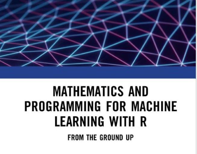
New R textbook for machine learning

Mathematics and Programming for Machine Learning with R -Chapter 2 Logic

Have a look at the FREE attached pdf of Chapter 2 on Logic and R from my recently published textbook,

Mathematics and Programming for Machine Learning with R: From the Ground Up, by William B. Claster (Author)
~430 pages, over 400 exercises.Mathematics and Programming for Machine Learning with R -Chapter 2 Logic
We discuss how to code machine learning algorithms in R but start from scratch. The first 4 chapters cover Logic, Sets, Probability, Functions. I am sharing Chapter 2 here on Logic and R here and will also probably release chapters 9 and 10 on Math for Neural Networks shortly. The text is on sale at Amazon here:
https://www.amazon.com/Mathematics-Programming-Machine-Learning-R-dp-0367507854/dp/0367507854/ref=mt_other?_encoding=UTF8&me=&qid=1623663440

I will try to add an errata page as well.