Create a hyper-marketing model using Naïve Bayes

By Huey Fern Tay with Greg Page

Everyone loves an extra income stream – even the super-wealthy owners of luxurious properties that they only inhabit for just a few weeks each year.  Offering a property as a short-term rental through a platform like Airbnb can provide a wonderful side hustle.  For some owners, however, the associated hassles could be a powerful deterrent to using the service.  Text messages at 3 a.m. about Wi-Fi passwords, stopped-up toilets, and the lack of water pressure in the shower might be just enough to tip the scales against such an undertaking…especially when such messages are followed up by angry “Why isn’t this fixed yet?” queries just 30 minutes later.

So what if an all-in-one concierge service could take away ALL of those hassles?  If an intermediary service could handle all of the tenant interactions, the marketing, the logistics of the key hand-offs, etc. then suddenly the idle rich jetsetters might be a bit more willing to open up their pied-a-terres to the unbathed masses.  Such a service would benefit all stakeholders – travelers would have more options, the property owners would earn more income, and the platform would receive more commission fees from the extra transactions. In exchange for a fee paid to the service, willing property owners could have a side hustle that was “all side, no hustle.”  

Let’s imagine that such a service is looking to establish itself, with an initial marketing outreach effort to high-end property owners not already using Airbnb.  Let’s also imagine that this new service is operating on a shoestring budget, and therefore needs to. How can it identify the properties within a city that are most likely to command high values in the short-term rental market? 

The Naïve Bayes classifier is a good candidate for the task at hand because of its simplicity, computational efficiency, and ability to handle categorical variables.  Furthermore, its classification outcomes come with associated probability values – we can use those to identify records that are most likely to belong to some particular group. 

To illustrate how this method could be used to solve the business problem outlined above, I will utilize Airbnb data of San Francisco listings.

One of the first decisions the modeler must make is deciding how to bin the data. In this case, the question is which numerical variable would you use to separate the properties? Would you use price, review ratings, or number of reviews? Each of these variables has a different impact on the outcome and may not be equally effective at separating classes. If the classes are not well separated, then even a large dataset will not be helpful.

The next important decision is to determine the number of classification categories you would like to create. Also, what would the cut-off be for each group? In other words, should you create four groups and bin them equally? Or should you create three groups by dividing the data according to a 15-70-15 proportion, 20-40-20, or 30-40-30…etc? The decision made at this step has a big impact on the model.

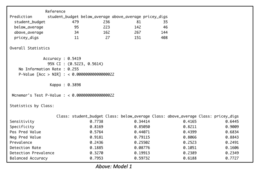
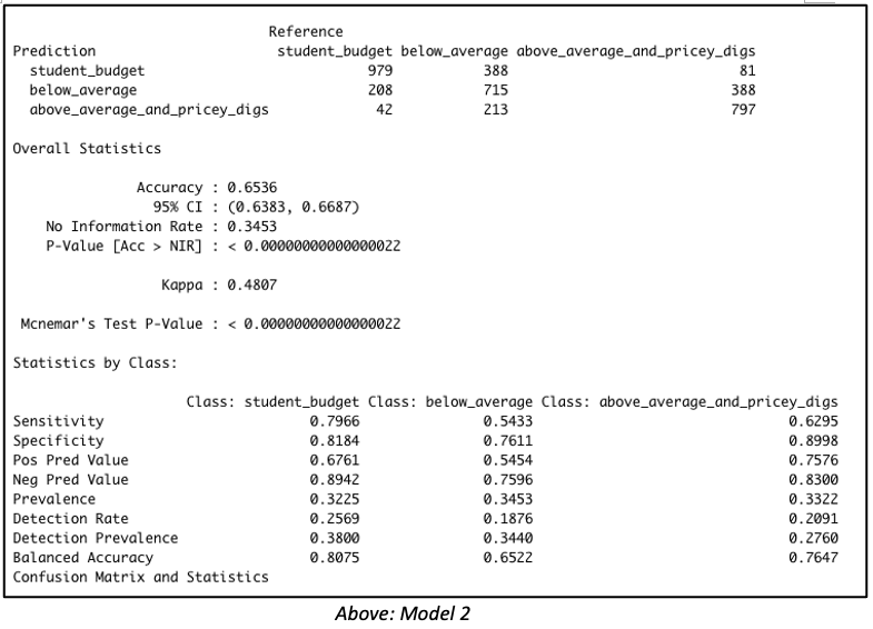
Consider both models below which were each created with 3811 rows of data representing 60% of the total dataset. Both models were created with the same predictor variables, such as the number of bedrooms, bathrooms, property type, location, etc. But in Model 1, the data was binned into 4 equal groups while in Model 2, the data was binned into 3 equal groups. The model summary for Model 1 showed the model has an accuracy of 54.19%, which is good considering that this performance is slightly more than double the No Information Rate (Naïve Rate). Model 2’s accuracy’s level is at 65.36%, a level which is nearly double its No Information Rate.

These are encouraging results but in our Airbnb example, we are more interested in knowing how well our model performs when it is asked to classify properties into any of the classes used in the model. For this reason, it is worth considering the true positive rate i.e. ‘sensitivity’. Model 1 is better at predicting the true positives (‘sensitivity’) for classes at opposite ends of the spectrum. This suggests Model 1 has difficulty reading nuances. On the other hand, Model 2’s performance in this regard is comparatively more balanced.


Naive Bayes model with four classification outcome


Naive Bayes output with three classification outcome


But wait – let’s get back to our original goal.  While overall accuracy is good to see, what we are most interested in here is identifying that high-end price group.  Owners of such units will be the best targets for our all-in-one concierge service.  Therefore, let’s dive a bit deeper to examine this model’s suitability for identifying such properties. 

By running the predict() function with the type=’raw’ parameter included, we can view the associated probabilities for each outcome class, and then rank records by probability of belonging to some particular outcome group. 

Taking this approach with the validation set, we find that among the 100 records identified by the model as most likely to land in the top tier group, 96 truly belonged to “Above Average and Pricey Digs.”   Among the 150 likeliest, 140 units, or 93.33%, actually belonged to that group, and among the 200 likeliest, 185 units, or 92.5%, were truly in that top tier. 

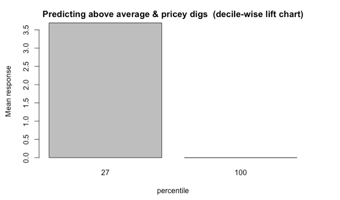
But that’s not all. It is worth going one step further by evaluating the model with lift charts or decile-wise lift charts because these charts determine how effectively our model ‘skims the cream’.

The decile-wise lift charts below illustrate how effectively the model can predict membership in the ‘above average and pricey digs’ group. When the model is used to classify the top 27% properties in this category, its performance is more than 3.5x better than a random guess.

Decile-wise lift chart shows the model is 3.5 times better at classifying the top 27 percent properties

Another way to assess the model’s ability to identify top-tier rentals is with a two-dimensional lift chart.  Such a chart only works with two-outcome class scenarios, so we start here by collapsing the first and second tiers together, and then labelling that group as “other.”  

Gains chart shows among the 500 records that the model says are most likely to land in the Above Average & Pricey Digs Tier, just over 400 truly did belong to that group

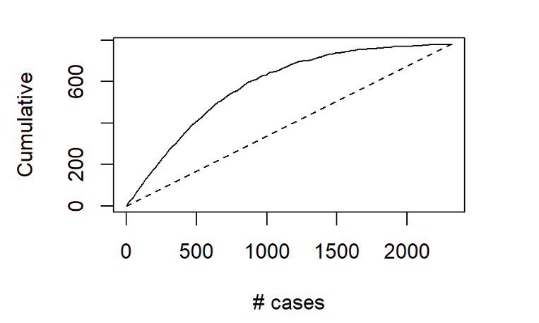
In the entire validation set, there are 780 units that land in the highest price tier.  The values along the x-axis represent all the validation set records, ranked in order of their probability of belonging to the highest-tier class.  The y-axis shows the number of correct predictions.  The solid line represents the model’s performance – it shows us, for instance, that among the 500 records that the model says are most likely to land in the Above Average & Pricey Digs Tier, just over 400 truly did belong to that group.  The line flattens out at around x=1500, because by that point, the model has already identified nearly all of the records that truly belonged to this outcome class. 

The dotted line, by contrast, shows how effective a model would be if it simply labelled all the records as belonging to the top tier.  Since 33.6%, of the validation records belong to this group, each x-axis value here corresponds to a y-axis value that is exactly 33.6% as large.  The difference between the solid line and the dotted line represents the model’s improvement as the number of cases increases.

What do these results mean for the concierge service?  Let’s revisit our original assumptions: 


  • such a service would most likely appeal to the owners of properties in the highest pricing tier;
  • the initial outreach efforts should be made to owners of properties not already registered with Airbnb; and that
  • the new service has a limited budget, and therefore needs to carefully focus its outreach efforts only on that tier of properties whose owners would be likeliest to use it
Given these assumptions, our primary interest does not lie with overall model accuracy.  The model’s ability to distinguish between the bottom two pricing tiers is almost immaterial to us; however, we are keenly interested in the answer to this question:  When the model predicts that a property will belong to the highest pricing tier, how often is it correct? 

As demonstrated here, the model delivers quite effectively in this regard, especially when we maintain a relatively narrow focus on the properties that are most likely to be top tier.  Splashy magazine inserts, Super Bowl advertisements, and big-ticket endorsements from celebrities might be in the cards for this service down the road, after it spreads across the globe and prepares for its IPO roadshow.  For now, though, the hyper-specific focus that can come from “skimming the cream” off the top of those Naïve Bayes model probability predictions may be the surest next step for this service’s success. 

Data source: Inside Airbnb
 

New R textbook for machine learning

Mathematics and Programming for Machine Learning with R -Chapter 2 Logic

Have a look at the FREE attached pdf of Chapter 2 on Logic and R from my recently published textbook,

Mathematics and Programming for Machine Learning with R: From the Ground Up, by William B. Claster (Author)
~430 pages, over 400 exercises.Mathematics and Programming for Machine Learning with R -Chapter 2 Logic
We discuss how to code machine learning algorithms in R but start from scratch. The first 4 chapters cover Logic, Sets, Probability, Functions. I am sharing Chapter 2 here on Logic and R here and will also probably release chapters 9 and 10 on Math for Neural Networks shortly. The text is on sale at Amazon here:
https://www.amazon.com/Mathematics-Programming-Machine-Learning-R-dp-0367507854/dp/0367507854/ref=mt_other?_encoding=UTF8&me=&qid=1623663440

I will try to add an errata page as well.

Understanding Naïve Bayes Classifier Using R

The Best Algorithms are the Simplest

The field of data science has progressed from simple linear regression models to complex ensembling techniques but the most preferred models are still the simplest and most interpretable. Among them are regression, logistic, trees and naive bayes techniques. Naive Bayes algorithm, in particular is a logic based technique which is simple yet so powerful that it is often known to outperform complex algorithms for very large datasets. Naive bayes is a common technique used in the field of medical science and is especially used for cancer detection. This article explains the underlying logic behind naive bayes algorithm and example implementation.

How Probability defines Everything

We calculate probability as the proportion of cases where an event happens and call it the probability of the event. Just as there is probability for a single event, we have probability of a group of events as the proportion of cases where the group of events occur together. Another concept in probability is calculating the occurrence of events in a particular sequence, that is, if it is known that something has already happened, what will be the probability that another event happens after that. By logic, one can understand that we are narrowing down our scope to only the case when that something has already happened and then calculating the proportion of cases where our second event occurs. To represent it mathematically, If A is the first event and B is the second event, then P(B|A) is our desired probability of calculating probability of event A after occurrence of event B, P(A n B) is probability of the two events occurring together

P(B | A) = P(B) * P(A | B) / P(A)

This is the foundation pillar for Naive bayes algorithm. Owing to this, Naive Bayes can handle different kind of events which are differentiated by the probabilities of event separately, that is , P(B) and conditional probability P(B|A). If the two probabilities are same, then it means that the occurrence of event A had no effect on event B and the events are known as independent events. If the conditional probability becomes zero, then it means the occurrence of event A implies that event B cannot occur. If the reverse is also true, then the events are known as mutually exclusive events and the occurrence of only one of the events at a time is possible. All other cases are classified as dependent events where the conditional probability can be either lower or higher than the original. In real life, every coin toss is independent of all other coin tosses made previously and thus coin tosses are independent. The outcome of a single coin toss is composed of mutually exclusive events. We cannot have a head and the tails at the same time. When we consider runs of multiple coin tosses, we are talking about dependent events. For a combination of three coin tosses, the final outcome is dependent of the first, second as well as the third coin toss.

How do we Calculate these Probabilities?

It is easy to calculate the probability of a single event. It equates to the number of cases when the event occurs divided by the total number of possible cases. For instance, the probability of a 6 in a single six-faced die roll is ⅙ if all the sides have equal chance of coming. However, one needs to be careful when calculating probabilities of two or more events. Simply knowing the probability of each event separately is not enough to calculate the probability of multiple events happening. If we additionally know that the events are independent, then the probability of them occurring together is the multiplication of each event separately.

We denote this mathematically as follows: P(A and B)=P(A)*P(B) – For independent events

As I already described, each coin toss is independent of other coin tosses. So the probability of having a Heads and a Heads combination in two coin tosses is P(Heads-Heads Combo)=P(Heads in first throw)*P(Heads in second throw)=½ * ½ = ¼

If the events are not independent, we can use the probability of any one event multiplied by the probability of second event after the first has happened
P(A and B)=P(A)*P(B|A) – For dependent events

An example of dependent events can be drawing cards without replacement. If you want to know that the two cards drawn are King and Queen then we know that the probability of the first event is dependent of 52 cards whereas the probability of the second event is dependent on 51 cards.

Thus, P(King and Queen)=P(King)*P(Queen|King)

Here, P(King) is 4/52. After a King is drawn, there are 4 queens out of 51 cards. So, P(Queen|King) is 4/51 P(King and Queen)=4/52*4/51=~0.6%

This is known as general multiplication rule. It also applies to the independent events scenario but since the events are independent, P(B|A) becomes equal to P(B)

The third case is for mutually exclusive events. If the events are mutually exclusive, we know that only one of the events can occur at a time. So the probability of the two events occurring together is zero. We are sometimes interested in probability of one of the events occuring and it is the sum of the individual probabilities in this scenario.

P(A OR B)=P(A)+P(B) – for mutually exclusive events

If we’re talking about a single six faced fair die throw, the probability of any two numbers occurring together is zero. In this case the probability of any prime number occuring is the sum of occurrence of each prime number. In this case P(2)+P(3)+P(5)

Had the events not been mutually exclusive, the probability of one of the events would have counted the probability of both events coming together twice. Hence we subtract this probability. P(A OR B)=P(A)+P(B)-P(A AND B) – for events which are not mutually exclusive

In a single six faced fair dice throw, the probability of throwing a multiple of 2 or 3 describes a scenario of events which are not mutually exclusive since 6 is both a multiple of 2 and 3 and is counted twice.

Thus, P(multiple of 2 or 3)=P(Multiple of 2)+P(Multiple of 3)- P(Multiple of 2 AND 3) =P(2,4,6)+P(3,6)-P(6)=3/6 + 2/6 -1/6 = 4/6 =2/3

This is known as general addition rule and similar to the multiplication rule, it also applies to the mutually exclusive events scenario but in that case, P(A AND B) is zero.

This is all we need to understand how Naive Bayes algorithm works. It takes into account all such scenarios and learns accordingly. Let’s get our hands dirty with a sample dataset.

Naive Bayes – a Not so Naive Algorithm

The reason that Naive Bayes algorithm is called Naive is not because it is simple or stupid. It is because the algorithm makes a very strong assumption about the data having features independent of each other while in reality, they may be dependent in some way. In other words, it assumes that the presence of one feature in a class is completely unrelated to the presence of all other features. If this assumption of independence holds, Naive Bayes performs extremely well and often better than other models. Naive Bayes can also be used with continuous features but is more suited to categorical variables. If all the input features are categorical, Naive Bayes is recommended. However, in case of numeric features, it makes another strong assumption which is that the numerical variable is normally distributed.

R supports a package called ‘e1071’ which provides the naive bayes training function. For this demonstration, we will use the classic titanic dataset and find out the cases which naive bayes can identify as survived.

The Titanic dataset in R is a table for about 2200 passengers summarised according to four factors – economic status ranging from 1st class, 2nd class, 3rd class and crew; gender which is either male or female; Age category which is either Child or Adult and whether the type of passenger survived. For each combination of Age, Gender, Class and Survived status, the table gives the number of passengers who fall into the combination. We will use the Naive Bayes Technique to classify such passengers and check how well it performs. As we know, Bayes theorem is based on conditional probability and uses the formula

P(A | B) = P(A) * P(B | A) / P(B)

We now know how this conditional probability comes from multiplication of events so if we use the general multiplication rule, we get another variation of the theorem that is, using P(A AND B) = P(A) * P(B | A), we can obtain the value for conditional probability: P(B | A) = P(A AND B) / P(A) which is the variation of Bayes theorem.

Since P(A AND B) also equals P(B) * P(A | B), we can substitute it and get back the original formula P(B | A) = P(B) * P(A | B) / P(A) Using this for each of the features among Age, Gender and Economic status, Naive Bayes algorithm will calculate the conditional probability of survival of the combination
#Getting started with Naive Bayes
#Install the package
#install.packages(“e1071”)
#Loading the library
library(e1071)
?naiveBayes #The documentation also contains an example implementation of Titanic dataset
#Next load the Titanic dataset
data(“Titanic”)
#Save into a data frame and view it
Titanic_df=as.data.frame(Titanic)
We see that there are 32 observations which represent all possible combinations of Class, Sex, Age and Survived with their frequency. Since it is summarised, this table is not suitable for modelling purposes. We need to expand the table into individual rows. Let’s create a repeating sequence of rows based on the frequencies in the table
#Creating data from table
repeating_sequence=rep.int(seq_len(nrow(Titanic_df)), Titanic_df$Freq) #This will repeat each combination equal to the frequency of each combination
#Create the dataset by row repetition created
Titanic_dataset=Titanic_df[repeating_sequence,]
#We no longer need the frequency, drop the feature
Titanic_dataset$Freq=NULL
The data is now ready for Naive Bayes to process. Let’s fit the model
#Fitting the Naive Bayes model
Naive_Bayes_Model=naiveBayes(Survived ~., data=Titanic_dataset)
#What does the model say? Print the model summary
Naive_Bayes_Model
Naive Bayes Classifier for Discrete Predictors
Call:
naiveBayes.default(x = X, y = Y, laplace = laplace)

A-priori probabilities:
Y
      No      Yes 
0.676965 0.323035 

Conditional probabilities:
     Class
Y          1st          2nd         3rd         Crew
  No    0.08187919  0.11208054  0.35436242  0.45167785
  Yes   0.28551336  0.16596343  0.25035162  0.29817159

     Sex
Y          Male         Female
  No    0.91543624  0.08456376
  Yes   0.51617440  0.48382560

     Age
Y         Child         Adult
  No    0.03489933  0.96510067
  Yes   0.08016878  0.91983122
The model creates the conditional probability for each feature separately. We also have the a-priori probabilities which indicates the distribution of our data. Let’s calculate how we perform on the data.
#Prediction on the dataset
NB_Predictions=predict(Naive_Bayes_Model,Titanic_dataset)
#Confusion matrix to check accuracy
table(NB_Predictions,Titanic_dataset$Survived)
NB_Predictions      No      Yes
                No      1364    362
                Yes     126     349
We have the results! We are able to classify 1364 out of 1490 “No” cases correctly and 349 out of 711 “Yes” cases correctly. This means the ability of Naive Bayes algorithm to predict “No” cases is about 91.5% but it falls down to only 49% of the “Yes” cases resulting in an overall accuracy of 77.8%

Conclusion: Can we Do any Better?

Naive Bayes is a parametric algorithm which implies that you cannot perform differently in different runs as long as the data remains the same. We will, however, learn another implementation of Naive Bayes algorithm using the ‘mlr’ package. Assuming the same session is going on for the readers, I will install and load the package and start fitting a model
#Getting started with Naive Bayes in mlr
#Install the package
#install.packages(“mlr”)
#Loading the library
library(mlr)
The mlr package consists of a lot of models and works by creating tasks and learners which are then trained. Let’s create a classification task using the titanic dataset and fit a model with the naive bayes algorithm.
#Create a classification task for learning on Titanic Dataset and specify the target feature
task = makeClassifTask(data = Titanic_dataset, target = "Survived")
#Initialize the Naive Bayes classifier
selected_model = makeLearner("classif.naiveBayes")
#Train the model
NB_mlr = train(selected_model, task)
The summary of the model which was printed in e3071 package is stored in learner model. Let’s print it and compare
#Read the model learned  
NB_mlr$learner.model
Naive Bayes Classifier for Discrete Predictors

Call:
naiveBayes.default(x = X, y = Y, laplace = laplace)

A-priori probabilities:
Y
      No      Yes 
0.676965 0.323035 

Conditional probabilities:
     Class
Y               1st         2nd         3rd         Crew
    No      0.08187919  0.11208054  0.35436242  0.45167785
    Yes     0.28551336  0.16596343  0.25035162  0.29817159

     Sex
Y               Male        Female
     No     0.91543624  0.08456376
    Yes     0.51617440  0.48382560

     Age
Y           Child       Adult
    No      0.03489933  0.96510067
    Yes     0.08016878  0.91983122
The a-priori probabilities and the conditional probabilities for the model are similar to the one calculated by e3071 package as was expected. This means that our predictions will also be the same.
#Predict on the dataset without passing the target feature
predictions_mlr = as.data.frame(predict(NB_mlr, newdata = Titanic_dataset[,1:3]))

##Confusion matrix to check accuracy
table(predictions_mlr[,1],Titanic_dataset$Survived)
        No      Yes
  No    1364    362
  Yes   126     349
As we see, the predictions are exactly same. The only way to improve is to have more features or more data. Perhaps, if we have more features such as the exact age, size of family, number of parents in the ship and siblings then we may arrive at a better model using Naive Bayes. In essence, Naive Bayes has an advantage of a strong foundation build and is very robust. I know of the ‘caret’ package which also consists of Naive Bayes function but it will also give us the same predictions and probability.

Author Bio:

This article was contributed by Perceptive Analytics. Madhur Modi, Chaitanya Sagar, Vishnu Reddy and Saneesh Veetil contributed to this article.

Perceptive Analytics provides data analytics, data visualization, business intelligence and reporting services to e-commerce, retail, healthcare and pharmaceutical industries. Our client roster includes Fortune 500 and NYSE listed companies in the USA and India.

Here is the Complete Code (used in this article):

#Getting started with Naive Bayes
#Install the package
#install.packages(“e1071”)
#Loading the library
library(e1071)
?naiveBayes #The documentation also contains an example implementation of Titanic dataset
#Next load the Titanic dataset
data("Titanic")
#Save into a data frame and view it
Titanic_df=as.data.frame(Titanic)
#Creating data from table
repeating_sequence=rep.int(seq_len(nrow(Titanic_df)), Titanic_df$Freq) #This will repeat each combination equal to the frequency of each combination

#Create the dataset by row repetition created
Titanic_dataset=Titanic_df[repeating_sequence,]
#We no longer need the frequency, drop the feature
Titanic_dataset$Freq=NULL

#Fitting the Naive Bayes model
Naive_Bayes_Model=naiveBayes(Survived ~., data=Titanic_dataset)
#What does the model say? Print the model summary
Naive_Bayes_Model

#Prediction on the dataset
NB_Predictions=predict(Naive_Bayes_Model,Titanic_dataset)
#Confusion matrix to check accuracy
table(NB_Predictions,Titanic_dataset$Survived)

#Getting started with Naive Bayes in mlr
#Install the package
#install.packages(“mlr”)
#Loading the library
library(mlr)

#Create a classification task for learning on Titanic Dataset and specify the target feature
task = makeClassifTask(data = Titanic_dataset, target = "Survived")

#Initialize the Naive Bayes classifier
selected_model = makeLearner("classif.naiveBayes")

#Train the model
NB_mlr = train(selected_model, task)

#Read the model learned  
NB_mlr$learner.model

#Predict on the dataset without passing the target feature
predictions_mlr = as.data.frame(predict(NB_mlr, newdata = Titanic_dataset[,1:3]))

##Confusion matrix to check accuracy
table(predictions_mlr[,1],Titanic_dataset$Survived)