I recently wrote a 80-page guide to how to get a programming job without a degree, curated from my experience helping students do just that at Springboard, a leading data science bootcamp. This excerpt is a part where I focus on an overview of the R programming language.
Description: R is an open-source programming language most often used by statisticians, data scientists, and academics who will use it to explore large data sets and distill insights from it. It offers multiple libraries that are useful for data processing tasks. Developed by John Chambers and other colleagues at Bell Laboratories, it is a refined version of its precursor language S.
It has strong libraries for data visualization, time series analysis and a variety of statistical analysis tasks.
It’s free software that runs on a variety of operating systems, from UNIX to Windows to OSX. It runs on the open source license of the GNU general public license and is thus free to use and adapt.
Salary: Median salaries for R users tend to vary, with the main split being the difference between data analysts who use R to query existing data pipelines and data scientists who build those data pipelines and train different models programmatically on top of larger data sets. The difference can be stark, with around a $90,000 median salary for data scientists who use R, vs about a $60,000 median salary for data analysts who use R.
Uses: R is often used to analyze datasets, especially in an academic context. Most frameworks that have evolved around R focus on different methods of data processing. The ggplot family of libraries has been widely recognized as some of the top programming modules for data visualization.
Differentiation: R is often compared to Python when it comes to data analysis and data science tasks. Its strong data visualization and manipulation libraries along with its data analysis-focused community help make it a strong contender for any data transformation, analysis, and visualization tasks.
Most Popular Github Projects:
1- Mal
Mal is a Clojure inspired lisp interpreter which can be implemented in the R programming language. With 4,500 stars, Mal requires one of the lowest amount of stars to qualify for the top repository of a programming language. It speaks to the fact that most of the open-source work done on the R programming language resides outside of Github.
2- Prophet
Prophet is a library that is able to do rich time series analysis by adjusting forecasts to account for seasonal and non-linear trends. It was created by Facebook and forms a part of the strong corpus of data analysis frameworks and libraries that exist for the R programming language.
3- ggplot2
Ggplot2 is a data visualization library for R that is based on the Grammar of Graphics. It is a library often used by data analysts and data scientists to display their results in charts, heatmaps, and more.
4- H2o-3
H2o-3 is the open source machine learning library for the R programming language, similar to scikit-learn for Python. It allows people using the R programming language to run deep learning and other machine learning techniques on their data, an essential utility in an era where data is not nearly as useful without machine learning techniques.
5- Shiny
Shiny is an easy web application framework for R that allows you to build interactive websites in a few lines of code without any JavaScript. It uses an intuitive UI (user interface) component based on Bootstrap. Shiny can take all of the guesswork out of building something for the web with the R programming language.
Example Sites: There are not many websites built with R, which is used more for data analysis tasks and projects that are internal to one computer. However, you can build things with R Markdown and build different webpages. You might also use a web development framework such as Shiny if you wanted to create simple interactive web applications around your data.
Frameworks: The awesome repository comes up again with a great list of different R packages and frameworks you can use. A few that are worth mentioning are packages such as dplyr that help you assemble data in an intuitive tabular fashion, ggplot2 to help with data visualization and plotly to help with interactive web displays of R analysis. R libraries and frameworks are some of the most robust for doing ad hoc data analysis and displaying the results in a variety of formats.
Learning Path: This article helps frame the resources you need to learn R, and how you should learn it, starting from syntax and going to specific packages. It makes for a great introduction to the field, even if you’re an absolute beginner. If you want to apply R to data science projects and different data analysis tasks, Datacamp will help you learn the skills and mentality you need to do just that — you’ll learn everything from machine learning practices with R to how to do proper data visualization of the results.
Resources: R-bloggers is a large community of R practitioners and writers who aim to share knowledge about R with each other. This list of 60+ resources on R can be used in case you ever get lost trying to learn R.
I hope this is helpful for you! Want more material like this? Check out my guide to how to get a programming job without a degree.
Category: R
R as learning tool: solving integrals

Integrals are so easy only math teachers could make them difficult.When I was in high school I really disliked math and, with hindsight, I would say it was just because of the the prehistoric teaching tools (when I saw this video I thought I’m not alone). I strongly believe that interaction CAUSES learning (I’m using “causes” here on purpose being quite aware of the difference between correlation and causation), practice should come before theory and imagination is not a skill you, as a teacher, could assume in your students. Here follows a short and simple practical explanation of integrals. The only math-thing I will write here is the following: f(x) = x + 7. From now on everything will be coded in R. So, first of all, what is a function? Instead of using the complex math philosophy let’s just look at it with a programming eye: it is a tool that takes something in input and returns something else as output. For example, if we use the previous tool with 2 as an input we get a 9. Easy peasy. Let’s look at the code:
# here we create the tool (called "f")
# it just takes some inputs and add it to 7
f <- function(x){x+7}

# if we apply it to 2 it returns a 9
f(2)
9
Then the second question comes by itself. What is an integral? Even simpler, it is just the sum of this tool applied to many inputs in a range. Quite complicated, let’s make it simpler with code:
# first we create the range of inputs
# basically x values go from 4 to 6
# with a very very small step (0.01)
# seq stands for sequence(start, end, step)
x <- seq(4, 6, 0.01)
x
4.00 4.01 4.02 4.03 4.04 4.05 4.06 4.07...

x[1]
4

x[2]
4.01
As you see, x has many values and each of them is indexed so it’s easy to find, e.g. the first element is 4 (x[1]). Now that we have many x values (201) within the interval from 4 to 6, we compute the integral.
# since we said that the integral is
# just a sum, let's call it IntSum and
# set it to the start value of 0
# in this way it will work as an accumulator
IntSum = 0Differently from the theory in which the calculation of the integral produces a new non-sense formula (just kidding, but this seems to be what math teachers are supposed to explain), the integral does produce an output, i.e. a number. We find this number by summing the output of each input value we get from the tool (e.g. 4+7, 4.01+7, 4.02+7, etc) multiplied by the step between one value and the following (e.g. 4.01-4, 4.02-4.01, 4.03-4.02, etc). Let’s clarify this, look down here:
# for each value of x
for(i in 2:201){

    # we do a very simple thing:
    # we cumulate with a sum
    # the output value of the function f
    # multiplied by each steps difference

    IntSum = IntSum + f(x[i])*(x[i]-x[i-1])


    # So for example,
    # with the first and second x values the numbers will be:
    #0.1101 = 0 + (4.01 + 7)*(4.01 - 4)

    # with the second and third:
    #0.2203 = 0.1101 + (4.02 + 7)*(4.02 - 4.01)

    # with the third and fourth:
    #0.3306 = 0.2203 + (4.03 + 7)*(4.03 - 4.02)

    # and so on... with the sum (integral) growing and growing
    # up until the last value
}

IntSum
24.01
Done! We have the integral but let’s have a look to the visualization of this because it can be represented and made crystal clear. Let’s add a short line of code to serve the purpose of saving the single number added to the sum each time. The reason why we decide to call it “bin” instead of, for example, “many_sum” will be clear in a moment.
# we need to store 201 calculation and we
# simply do what we did for IntSum but 201 times
bin = rep(0, 201)
bin
0 0 0 0 0 0 0 0 0 0 0 0 ...
Basically, we created a sort of memory to host each of the calculation as you see down here:
for (i in 2:201){

    # the sum as earlier
    IntSum = IntSum + f(x[i])*(x[i]-x[i-1])

    # overwrite each zero with each number
    bin[i] = f(x[i])*(x[i]-x[i-1])
}

IntSum
24.01

bin
0.0000 0.1101 0.1102 0.1103 0.1104 0.1105 ..

sum(bin)
24.01
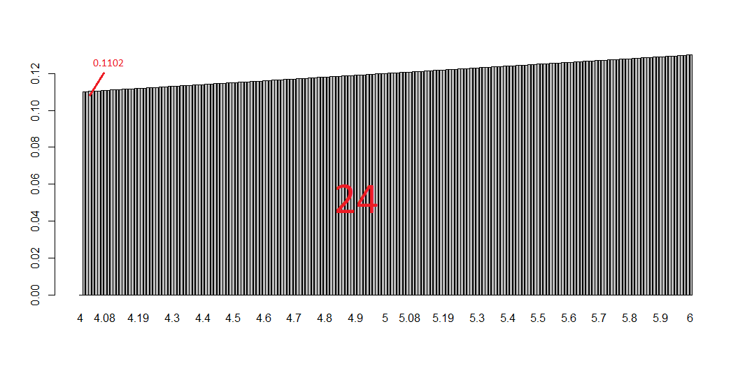
Now if you look at the plot below you get the whole story: each bin is a tiny bar with a very small area and is the smallest part of the integral (i.e. the sum of all the bins).
# plotting them all
barplot(bin, names.arg=x)
This post is also shared in https://www.linkedin.com/
Using Shiny Dashboards for Financial Analysis
For some time now, I have been trading traditional assets—mostly U.S. equities. About a year ago, I jumped into the cryptocurrency markets to try my hand there as well. In my time in investor Telegram chats and subreddits, I often saw people arguing over which investments had performed better over time, but the reality was that most such statements were anecdotal, and thus unfalsifiable.
Given the paucity of cryptocurrency data available in an easily accessible format, it was quite difficult to say for certain that a particular investment was a good one relative to some alternative, unless you were very familiar with a handful of APIs. Even then, assuming you knew how to get daily OHLC data for a crypto-asset like Bitcoin, in order to compare it to some other asset—say Amazon stock—you would have to eyeball trends from a website like Yahoo finance or scrape that data separately and build your own visualizations and metrics. In short, historical asset performance comparisons in the crypto space were difficult to conduct for all but the most technically savvy individuals, so I set out to build a tool that would remedy this, and the Financial Asset Comparison Tool was born.
In this post, I aim to describe a few key components of the dashboard, and also call out lessons learned from the process of iterating on the tool along the way. Prior to proceeding, I highly recommend that you read the app’s README and take a look at the UI and code base itself, as this will provide the context necessary to understanding the rest of the commentary below.
I’ll start by delving into a few principles that I find to be to key when designing analytic dashboards, drawing on the asset comparison dashboard as my exemplar, and will end with some discussion of the relative utility of a few packages integral to the app. Overall, my goal is not to focus on the tool that I built alone, but to highlight a few main best practices when it comes to building dashboards for any analysis.
Build the app around the story, not the other way around.
Before ever writing a single line of code for an analytic app, I find that it is absolutely imperative to have a clear vision of the story that the tool must tell. I do not mean by this that you should already have conclusions about your data that you will then force the app into telling, but rather, that you must know how you want your user to interact with the app in order glean useful information.
In the case of my asset comparison tool, I wanted to serve multiple audiences—everyone from a casual trader who just wanted to see which investment produced the greatest net profit over a period of time, to a more experience trader, who had more nuanced questions about risk-adjusted return on investment given varying discount rates. The trick is thus building the app in such a way that serves all possible audiences without hindering any one type of user in particular.
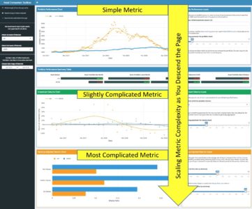
The way I designed my app to meet this need was to build the UI such that as you descend the various sections vertically, the metrics displayed scale in complexity. My reasoning for this becomes apparent when you consider the two extremes in terms of users—the most basic vs. the most advanced trader.
The most basic user will care only about the assets of interest, the time period they want to examine, and how their initial investment performed over time. As such, they will start with the sidebar, input their assets and time frame of choice, and then use the top right-most input box to modulate their initial investment amount (although some may choose to stick with the default value here). They will then see the first chart change to reflect their choices, and they will see, both visually, and via the summary table below, which asset performed better.
The experienced trader, on the other hand, will start off exactly as the novice did, by choosing assets of interest, a time frame of reference, and an initial investment amount. They may then choose to modulate the LOESS parameters as they see fit, descending the page, looking over the simple returns section, perhaps stopping to make changes to the corresponding inputs there, and finally ending at the bottom of the page—at the Sharpe Ratio visualizations. Here they will likely spend more time—playing around with the time period over which to measure returns and changing the risk-free rate to align with their own personal macroeconomic assumptions.
The point of these two examples is to illustrate that the app by dint of its structure alone guides the user through the analytic story in a waterfall-like manner—building from simple portfolio performance, to relative performance, to the most complicated metrics for risk-adjusted returns. This keeps the novice trader from being overwhelmed or confused, and also allows the most experienced user to follow the same line of thought that they would anyway when comparing assets, while following a logical progression of complexity, as shown via the screenshot below.
Once you think you have a structure that guides all users through the story you want them to experience, test it by asking yourself if the app flows in such a way that you could pose and answer a logical series of questions as you navigate the app without any gaps in cohesion. In the case of this app, the questions that the UI answers as you descend are as follows:
Thus, when you string these questions together, you can make statements of the type: “Asset X seemed to outperform Asset Y in terms of absolute profit, and this trend held true as well when it comes to simple return on investment, over varying time frames. That said, when you take into account the variance inherent to Asset X, it seems that Asset Y may have been the best choice, as the excess downside risk associated with Asset X outweighs its excess net profitability.
Too many cooks in the kitchen—the case for a functional approach to app-building.
While the design of the UI of any analytic app is of great importance, it’s important to not forget that the code base itself should also be well-designed; a fully-functional app from the user’s perspective can still be a terrible app to work with if the code is a jumbled, incomprehensible mess. A poorly designed code base makes QC a tiresome, aggravating process, and knowledge sharing all but impossible.
For this reason, I find that sourcing a separate R script file containing all analytic functions necessitated by the app is the best way to go, as done below (you can see Functions.R at my repo here).
Not only does this allow for a more comprehensible and less-cluttered App.R, but it also drastically improves testability and reusability of the code. Consider the example function below, used to create the portfolio performance chart in the app (first box displayed in the UI, center middle).
Writing this function in the sourced Functions.R file instead of directly within the App.R allows for the developer to first test the function itself with fake data—i.e. data not gleaned from the reactive inputs. Once it has been tested in this way, it can be integrated in the app.R on the server side as shown below, with very little code.
This process allows for better error-identification and troubleshooting. If, for example, you want to change the work accomplished by the analytic function in some way, you can make the changes necessary to the code, and if the app fails to produce the desired outcome, you simply restart the chain: first you test the function in a vacuum outside of the app, and if it runs fine there, then you know that you have a problem with the way the reactive inputs are integrating with the function itself. This is a huge time saver when debugging.
Lastly, this allows for ease of reproducibility and hand-offs. If, say, one of your functions simply takes in a dataset and produces a chart of some sort, then it can be easily copied from the Functions.R and reused elsewhere. I have done this too many times to count, ripping code from project and, with a few alterations, instantly applying it in other contexts. This is easy to do if the functions are written in a manner not dependent on a particular Shiny reactive structure. For all these reasons, it makes sense in most cases to keep the code for the app UI and inputs cleanly separated from the analytic functions via a sourced R script.
Dashboard documentation—both a story and a manual, not one or the other.
When building an app for a customer at work, I never simply write an email with a link in it and write “here you go!” That will result in, at best, a steep learning curve, and at worst, an app used in an unintended way, resulting in user frustration or incorrect results. I always meet with the customer, explain the purpose and functionalities of the tool, walk through the app live, take feedback, and integrate any key takeaways into further iterations.
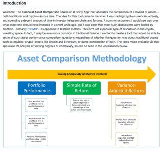
Even if you are just planning on writing some code to put up on GitHub, you should still consider all of these steps when working on the documentation for your app. In most cases, the README is the epicenter of your documentation—the README is your meeting with the customer. As you saw when reading the README for the Asset Comparison Tool, I always start my READMEs with a high-level introduction to the purpose of the app—hopefully written or supplemented with visuals (as seen below) that are easy to understand and will capture the attention of browsing passers-by.
After this introduction, the rest of the potential sections to include can vary greatly from app-to-app. In some cases apps are meant to answer one particular question, and might have a variety of filters or supplemental functionalities—one such example can be found here. As can be seen, in that README, I spend a great deal of time on the methodology after making the overall purpose clear, calling out additional options along the way. In the case of the README for the Asset Comparison Tool, however, the story is a bit different. Given that there are many questions that the app seeks to answer, it makes sense to answer each in turn, writing the README in such a way that its progression mirrors the logical flow of the progression intended for the app’s user.
One should of course not neglect to cover necessary technical information in the README as well. Anything that is not immediately clear from using the app should be clarified in the README—from calculation details to the source of your data, etc. Finally, don’t neglect the iterative component! Mention how you want to interact with prospective users and collaborators in your documentation. For example, I normally call out how I would like people to use the Issues tab on GitHub to propose any changes or additions to the documentation, or the app in general. In short, your documentation must include both the story you want to tell, and a manual for your audience to follow.
Why Shiny Dashboard?
One of the first things you will notice about the app.R code is that the entire thing is built using Shiny Dashboard as its skeleton. There are a two main reasons for this, which I will touch on in turn.
Shiny Dashboard provides the biggest bang for your buck in terms of how much UI complexity and customizability you get out of just a small amount of code.
I can think of few cases where any analyst or developer would prefer longer, more verbose code to a shorter, succinct solution. That said, Shiny Dashboard’s simplicity when it comes to UI manipulation and customization is not just helpful because it saves you time as a coder, but because it is intuitive from the perspective of your audience.
Most of the folks that use the tools I have built to shed insight into economic questions don’t know how to code in R or Python, but they can, with a little help from extensive commenting and detailed documentation, understand the broad structure of an app coded in Shiny Dashboard format. This is, I believe, largely a function of two features of Shiny Dashboard: the colloquial-English-like syntax of the code for UI elements, and the lack of the necessity for in-line or external CSS.
As you can see from the example below, Shiny Dashboard’s system of “boxes” for UI building is easy to follow. Users can see a box in the app and easily tie that back to a particular box in the UI code.
Here is the box as visible to the user:
And here is the code that produces the box:
Secondly, and somewhat related to the first point, with Shiny Dashboard, much of the coloring and overall UI design comes pre-made via dashboard-wide “skins”, and box-specific “statuses.”
This is great if you are okay sacrificing a bit of control for a significant reduction in code complexity. In my experience dealing with non-coding-proficient audiences, I find that in-line CSS or complicated external CSS makes folks far more uncomfortable with the code in general. Anything you can do to reduce this anxiety and make those using your tools feel as though they understand them better is a good thing, and Shiny Dashboard makes that easier.
Shiny Dashboard’s combination of sidebar and boxes makes for easy and efficient data processing when your app has a waterfall-like analytic structure.
Having written versions of this app both in base Shiny and using Shiny Dashboard, the number one reason I chose Shiny Dashboard was the fact that the analytic questions I sought to solve followed a waterfall-like structure, as explained in the previous section. This works perfectly well with Shiny Dashboard’s combination of sidebar input controls and inputs within UI boxes themselves.
The inputs of primordial importance to all users are included in the sidebar UI: the two assets to analyze, and the date range over which to compare their performance. These are the only inputs that all users, regardless of experience or intent, must absolutely use, and when they are changed, all views in the dashboard will be affected. All other inputs are stored in the UI Boxes adjacent to the views that they modulate. This makes for a much more intuitive and fluid user experience, as once the initial sidebar inputs have been modulated, the sidebar can be hidden, as all other non-hidden inputs affect only the visualizations to which they are adjacent.
This waterfall-like structure also makes for more efficient reactive processes on the Shiny back-end. The inputs on the sidebar are parameters that, when changed, force the main reactive function that creates that primary dataset to fire, thus recreating the base dataset (as can be seen in the code for that base datasets creation below).
Each of the visualizations are then produced via their own separate reactive functions, each of which takes as an input the main reactive (as shown below). This makes it so that whenever the sidebar inputs are changed, all reactives fire and all visualizations are updated; however, if all that is changed is a single loess smoothing parameter input, only the reactive used in the creation of that particular parameter-dependent visualization fires, which makes for great computational efficiency.
Why Plotly?
Plotly vs. ggplot is always a fun subject for discussion among folks who build visualizations in R. Sometimes I feel like such discussions just devolve into the same type of argument as R vs. Python for data science (my answer to this question being just pick one and learn it well), but over time I have found that there are actually some circumstances where the plotly vs. ggplot debate can yield cleaner answers.
In particular, I have found in working on this particular type of analytic app that there are two areas where plotly has a bit of an advantage: clickable interactivity, and wide data.
Those familiar with ggplot will know that every good ggplot begins with long data. It is possible, via some functions, to transform wide data into a long format, but that transformation can sometimes be problematic. While there are essentially no circumstances in which it is impossible to transform wide data into long format, there are a handful of cases where it is excessively cumbersome: namely, when dealing with indexed xts objects (as shown below) or time series / OHLC-styled data.
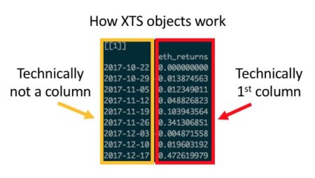
In these cases—either due to the sometimes-awkward way in which you have to handle rowname indexes in xts, or the time and code complexity saved by not having to transform every dataset into long format—plotly offers efficiency gains relative to ggplot.
The aforementioned efficiency gains are a reason to choose plotly in some cases because it makes the life of the coder easier, but there are also reasons why it sometimes make the life of the user easier as well.
If one of the primary utilities of a visualization is to allow the user the ability to seamlessly and intuitively zoom in on, select, or filter the data displayed, particularly in the context of a Shiny App, then plotly should be strongly considered. Sure, ggplotly wrappers can be used to make a ggplot interactive, but with an added layer of abstraction comes an added layer of possible errors. While in most cases a ggplotly wrapper should work seamlessly, I have found that, particularly in cases where auto-sizing and margin size specification is key, ggplotly can require a great deal of added code in order to work correctly in a Shiny context.
In summary, when considering when to start with plotly vs. when to start with ggplot, I find one question to be particularly helpful: what do I value most—visual complexity and/or customization, or interactive versatility and/or preserving wide data?
If I choose the former, then ggplot is what I need; otherwise, I go with plotly. More often than not I find that ggplot emerges victorious, but even if you disagree with me in my decision-making calculus, I think it is helpful to at least think through what your personal calculus is. This will save you time when coding, as instead of playing around with various types of viz, you can simply pose the question(s) behind your calculus and know quickly what solution best fits your problem.
Why Formattable?
The case for formattable is, in my opinion, a much easier case to make than arguing for plotly vs. ggplot. The only question worth asking when deciding on whether or not to use formattable in your app is: do I want my table to tell a quick story via added visual complexity within the same cell that contains my data, or is a reference table all I am looking for? If you chose the former, formattable is probably a good way to go. You’ll notice as well that the case for formattable is very specific–in most cases there is likely a simpler solution via the DT or kableExtra packages.
The one downside that I have encountered in dealing with formattable code is the amount of code necessary to generate even moderately complicated tables. That said, this problem is easily remedied via a quick function that we can use to kill most of the duplicative coding, as seen in the example below.
First, here is the long form version:
This code can easily be shortened via the integration of a custom function, as shown below.
As can be seen, formattable allows for a great deal of added complexity in crafting your table—complexity that may not be suited for all apps. That said, if you do want to quickly draw a user’s attention to something in a table, formattable is a great solution, and most of the details of the code can be greatly simplified via a function, as shown.
Conclusions:
That was a lot—I know—but I hope that from this commentary and my exemplar of the Asset Comparison Tool more generally has helped to inform your understanding of how dashboards can serve as a helpful analytic tool. Furthermore, I hope to have prompted some thoughts as to the best practices to be followed when building such a tool. I’ll end with a quick tl;dr:
Thanks for reading!
Given the paucity of cryptocurrency data available in an easily accessible format, it was quite difficult to say for certain that a particular investment was a good one relative to some alternative, unless you were very familiar with a handful of APIs. Even then, assuming you knew how to get daily OHLC data for a crypto-asset like Bitcoin, in order to compare it to some other asset—say Amazon stock—you would have to eyeball trends from a website like Yahoo finance or scrape that data separately and build your own visualizations and metrics. In short, historical asset performance comparisons in the crypto space were difficult to conduct for all but the most technically savvy individuals, so I set out to build a tool that would remedy this, and the Financial Asset Comparison Tool was born.
In this post, I aim to describe a few key components of the dashboard, and also call out lessons learned from the process of iterating on the tool along the way. Prior to proceeding, I highly recommend that you read the app’s README and take a look at the UI and code base itself, as this will provide the context necessary to understanding the rest of the commentary below.
I’ll start by delving into a few principles that I find to be to key when designing analytic dashboards, drawing on the asset comparison dashboard as my exemplar, and will end with some discussion of the relative utility of a few packages integral to the app. Overall, my goal is not to focus on the tool that I built alone, but to highlight a few main best practices when it comes to building dashboards for any analysis.
Build the app around the story, not the other way around.
Before ever writing a single line of code for an analytic app, I find that it is absolutely imperative to have a clear vision of the story that the tool must tell. I do not mean by this that you should already have conclusions about your data that you will then force the app into telling, but rather, that you must know how you want your user to interact with the app in order glean useful information.
In the case of my asset comparison tool, I wanted to serve multiple audiences—everyone from a casual trader who just wanted to see which investment produced the greatest net profit over a period of time, to a more experience trader, who had more nuanced questions about risk-adjusted return on investment given varying discount rates. The trick is thus building the app in such a way that serves all possible audiences without hindering any one type of user in particular.
The way I designed my app to meet this need was to build the UI such that as you descend the various sections vertically, the metrics displayed scale in complexity. My reasoning for this becomes apparent when you consider the two extremes in terms of users—the most basic vs. the most advanced trader.
The most basic user will care only about the assets of interest, the time period they want to examine, and how their initial investment performed over time. As such, they will start with the sidebar, input their assets and time frame of choice, and then use the top right-most input box to modulate their initial investment amount (although some may choose to stick with the default value here). They will then see the first chart change to reflect their choices, and they will see, both visually, and via the summary table below, which asset performed better.
The experienced trader, on the other hand, will start off exactly as the novice did, by choosing assets of interest, a time frame of reference, and an initial investment amount. They may then choose to modulate the LOESS parameters as they see fit, descending the page, looking over the simple returns section, perhaps stopping to make changes to the corresponding inputs there, and finally ending at the bottom of the page—at the Sharpe Ratio visualizations. Here they will likely spend more time—playing around with the time period over which to measure returns and changing the risk-free rate to align with their own personal macroeconomic assumptions.
The point of these two examples is to illustrate that the app by dint of its structure alone guides the user through the analytic story in a waterfall-like manner—building from simple portfolio performance, to relative performance, to the most complicated metrics for risk-adjusted returns. This keeps the novice trader from being overwhelmed or confused, and also allows the most experienced user to follow the same line of thought that they would anyway when comparing assets, while following a logical progression of complexity, as shown via the screenshot below.
Once you think you have a structure that guides all users through the story you want them to experience, test it by asking yourself if the app flows in such a way that you could pose and answer a logical series of questions as you navigate the app without any gaps in cohesion. In the case of this app, the questions that the UI answers as you descend are as follows:
- How do these assets compare in terms of absolute profit?
- How do these assets compare in terms of simple return on investment?
- How do these assets compare in terms of variance-adjusted and/or risk-adjusted return on investment?
Thus, when you string these questions together, you can make statements of the type: “Asset X seemed to outperform Asset Y in terms of absolute profit, and this trend held true as well when it comes to simple return on investment, over varying time frames. That said, when you take into account the variance inherent to Asset X, it seems that Asset Y may have been the best choice, as the excess downside risk associated with Asset X outweighs its excess net profitability.
Too many cooks in the kitchen—the case for a functional approach to app-building.
While the design of the UI of any analytic app is of great importance, it’s important to not forget that the code base itself should also be well-designed; a fully-functional app from the user’s perspective can still be a terrible app to work with if the code is a jumbled, incomprehensible mess. A poorly designed code base makes QC a tiresome, aggravating process, and knowledge sharing all but impossible.
For this reason, I find that sourcing a separate R script file containing all analytic functions necessitated by the app is the best way to go, as done below (you can see Functions.R at my repo here).
# source the Functions.R file, where all analytic functions for the app are stored
source("Functions.R")
Not only does this allow for a more comprehensible and less-cluttered App.R, but it also drastically improves testability and reusability of the code. Consider the example function below, used to create the portfolio performance chart in the app (first box displayed in the UI, center middle).
build_portfolio_perf_chart <- function(data, port_loess_param = 0.33){

  port_tbl <- data[,c(1,4:5)]

  # grabbing the 2 asset names
  asset_name1 <- sub('_.*', '', names(port_tbl)[2])
  asset_name2 <- sub('_.*', '', names(port_tbl)[3])

  # transforms dates into correct type so smoothing can be done
  port_tbl[,1] <- as.Date(port_tbl[,1])
  date_in_numeric_form <- as.numeric((port_tbl[,1]))
  # assigning loess smoothing parameter
  loess_span_parameter <- port_loess_param

  # now building the plotly itself
  port_perf_plot <- plot_ly(data = port_tbl, x = ~port_tbl[,1]) %>%
    # asset 1 data plotted
    add_markers(y =~port_tbl[,2],
                marker = list(color = '#FC9C01'),
                name = asset_name1,
                showlegend = FALSE) %>%
    add_lines(y = ~fitted(loess(port_tbl[,2] ~ date_in_numeric_form, span = loess_span_parameter)),
              line = list(color = '#FC9C01'),
              name = asset_name1,
              showlegend = TRUE) %>%
    # asset 2 data plotted
    add_markers(y =~port_tbl[,3],
                marker = list(color = '#3498DB'),
                name = asset_name2,
                showlegend = FALSE) %>%
    add_lines(y = ~fitted(loess(port_tbl[,3] ~ date_in_numeric_form, span = loess_span_parameter)),
              line = list(color = '#3498DB'),
              name = asset_name2,
              showlegend = TRUE) %>%
    layout(
      title = FALSE,
      xaxis = list(type = "date",
                   title = "Date"),
      yaxis = list(title = "Portfolio Value ($)"),
      legend = list(orientation = 'h',
                    x = 0,
                    y = 1.15)) %>%
    add_annotations(
      x= 1,
      y= 1.133,
      xref = "paper",
      yref = "paper",
      text = "",
      showarrow = F
    )

  return(port_perf_plot)

}
Writing this function in the sourced Functions.R file instead of directly within the App.R allows for the developer to first test the function itself with fake data—i.e. data not gleaned from the reactive inputs. Once it has been tested in this way, it can be integrated in the app.R on the server side as shown below, with very little code.
  output$portfolio_perf_chart <-
    debounce(
      renderPlotly({
        data <- react_base_data()
        build_portfolio_perf_chart(data, port_loess_param = input$port_loess_param)
      }),
      millis = 2000) # sets wait time for debounce
This process allows for better error-identification and troubleshooting. If, for example, you want to change the work accomplished by the analytic function in some way, you can make the changes necessary to the code, and if the app fails to produce the desired outcome, you simply restart the chain: first you test the function in a vacuum outside of the app, and if it runs fine there, then you know that you have a problem with the way the reactive inputs are integrating with the function itself. This is a huge time saver when debugging.
Lastly, this allows for ease of reproducibility and hand-offs. If, say, one of your functions simply takes in a dataset and produces a chart of some sort, then it can be easily copied from the Functions.R and reused elsewhere. I have done this too many times to count, ripping code from project and, with a few alterations, instantly applying it in other contexts. This is easy to do if the functions are written in a manner not dependent on a particular Shiny reactive structure. For all these reasons, it makes sense in most cases to keep the code for the app UI and inputs cleanly separated from the analytic functions via a sourced R script.
Dashboard documentation—both a story and a manual, not one or the other.
When building an app for a customer at work, I never simply write an email with a link in it and write “here you go!” That will result in, at best, a steep learning curve, and at worst, an app used in an unintended way, resulting in user frustration or incorrect results. I always meet with the customer, explain the purpose and functionalities of the tool, walk through the app live, take feedback, and integrate any key takeaways into further iterations.
Even if you are just planning on writing some code to put up on GitHub, you should still consider all of these steps when working on the documentation for your app. In most cases, the README is the epicenter of your documentation—the README is your meeting with the customer. As you saw when reading the README for the Asset Comparison Tool, I always start my READMEs with a high-level introduction to the purpose of the app—hopefully written or supplemented with visuals (as seen below) that are easy to understand and will capture the attention of browsing passers-by.
After this introduction, the rest of the potential sections to include can vary greatly from app-to-app. In some cases apps are meant to answer one particular question, and might have a variety of filters or supplemental functionalities—one such example can be found here. As can be seen, in that README, I spend a great deal of time on the methodology after making the overall purpose clear, calling out additional options along the way. In the case of the README for the Asset Comparison Tool, however, the story is a bit different. Given that there are many questions that the app seeks to answer, it makes sense to answer each in turn, writing the README in such a way that its progression mirrors the logical flow of the progression intended for the app’s user.
One should of course not neglect to cover necessary technical information in the README as well. Anything that is not immediately clear from using the app should be clarified in the README—from calculation details to the source of your data, etc. Finally, don’t neglect the iterative component! Mention how you want to interact with prospective users and collaborators in your documentation. For example, I normally call out how I would like people to use the Issues tab on GitHub to propose any changes or additions to the documentation, or the app in general. In short, your documentation must include both the story you want to tell, and a manual for your audience to follow.
Why Shiny Dashboard?
One of the first things you will notice about the app.R code is that the entire thing is built using Shiny Dashboard as its skeleton. There are a two main reasons for this, which I will touch on in turn.
Shiny Dashboard provides the biggest bang for your buck in terms of how much UI complexity and customizability you get out of just a small amount of code.
I can think of few cases where any analyst or developer would prefer longer, more verbose code to a shorter, succinct solution. That said, Shiny Dashboard’s simplicity when it comes to UI manipulation and customization is not just helpful because it saves you time as a coder, but because it is intuitive from the perspective of your audience.
Most of the folks that use the tools I have built to shed insight into economic questions don’t know how to code in R or Python, but they can, with a little help from extensive commenting and detailed documentation, understand the broad structure of an app coded in Shiny Dashboard format. This is, I believe, largely a function of two features of Shiny Dashboard: the colloquial-English-like syntax of the code for UI elements, and the lack of the necessity for in-line or external CSS.
As you can see from the example below, Shiny Dashboard’s system of “boxes” for UI building is easy to follow. Users can see a box in the app and easily tie that back to a particular box in the UI code.
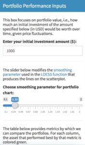
Here is the box as visible to the user:
And here is the code that produces the box:
box(
        title = "Portfolio Performance Inputs",
        status= "primary",
        solidHeader = TRUE,
        h5("This box focuses on portfolio value, i.e., how much an initial investment of the amount specified below (in USD) would be worth over time, given price fluctuations."),

        textInput(
          inputId = "initial_investment",
          label = "Enter your initial investment amount ($):",
          value = "1000"),

        hr(),

        h5("The slider below modifies the", a(href = "https://stats.stackexchange.com/questions/2002/how-do-i-decide-what-span-to-use-in-loess-regression-in-r", "smoothing parameter"), "used in the", a(href = "https://en.wikipedia.org/wiki/Local_regression", "LOESS function"), "that produces the lines on the scatterplot."),

        sliderInput(
          inputId = "port_loess_param",
          label = "Smoothing parameter for portfolio chart:",
          min = 0.1,
          max = 2,
          value = .33,
          step = 0.01,
          animate = FALSE
        ),

        hr(),
        h5("The table below provides metrics by which we can compare the portfolios. For each column, the asset that performed best by that metric is colored green."),

        height = 500,
        width = 4
      )
Secondly, and somewhat related to the first point, with Shiny Dashboard, much of the coloring and overall UI design comes pre-made via dashboard-wide “skins”, and box-specific “statuses.”
This is great if you are okay sacrificing a bit of control for a significant reduction in code complexity. In my experience dealing with non-coding-proficient audiences, I find that in-line CSS or complicated external CSS makes folks far more uncomfortable with the code in general. Anything you can do to reduce this anxiety and make those using your tools feel as though they understand them better is a good thing, and Shiny Dashboard makes that easier.
Shiny Dashboard’s combination of sidebar and boxes makes for easy and efficient data processing when your app has a waterfall-like analytic structure.
Having written versions of this app both in base Shiny and using Shiny Dashboard, the number one reason I chose Shiny Dashboard was the fact that the analytic questions I sought to solve followed a waterfall-like structure, as explained in the previous section. This works perfectly well with Shiny Dashboard’s combination of sidebar input controls and inputs within UI boxes themselves.
The inputs of primordial importance to all users are included in the sidebar UI: the two assets to analyze, and the date range over which to compare their performance. These are the only inputs that all users, regardless of experience or intent, must absolutely use, and when they are changed, all views in the dashboard will be affected. All other inputs are stored in the UI Boxes adjacent to the views that they modulate. This makes for a much more intuitive and fluid user experience, as once the initial sidebar inputs have been modulated, the sidebar can be hidden, as all other non-hidden inputs affect only the visualizations to which they are adjacent.
This waterfall-like structure also makes for more efficient reactive processes on the Shiny back-end. The inputs on the sidebar are parameters that, when changed, force the main reactive function that creates that primary dataset to fire, thus recreating the base dataset (as can be seen in the code for that base datasets creation below).
  # utility functions to be used within the server; this enables us to use a textinput for our portfolio values
  exists_as_number <- function(item) {
    !is.null(item) && !is.na(item) && is.numeric(item)
  }

  # data-creation reactives (i.e. everything that doesn't directly feed an output)

  # first is the main data pull which will fire whenever the primary inputs (asset_1a, asset_2a, initial_investment, or port_dates1a change)
  react_base_data <- reactive({
    if (exists_as_number(as.numeric(input$initial_investment)) == TRUE) {
      # creates the dataset to feed the viz
      return(
        get_pair_data(
          asset_1 = input$asset_1a,
          asset_2 = input$asset_2a,
          port_start_date = input$port_dates1a[1],
          port_end_date = input$port_dates1a[2],
          initial_investment = (as.numeric(input$initial_investment))
        )
      )
    } else {
      return(
        get_pair_data(
          asset_1 = input$asset_1a,
          asset_2 = input$asset_2a,
          port_start_date = input$port_dates1a[1],
          port_end_date = input$port_dates1a[2],
          initial_investment = (0)
        )
      )
    }
  })
Each of the visualizations are then produced via their own separate reactive functions, each of which takes as an input the main reactive (as shown below). This makes it so that whenever the sidebar inputs are changed, all reactives fire and all visualizations are updated; however, if all that is changed is a single loess smoothing parameter input, only the reactive used in the creation of that particular parameter-dependent visualization fires, which makes for great computational efficiency.
 # Now the reactives for the actual visualizations
  output$portfolio_perf_chart <-
    debounce(
      renderPlotly({
        data <- react_base_data()
        build_portfolio_perf_chart(data, port_loess_param = input$port_loess_param)
      }),
      millis = 2000) # sets wait time for debounce
Why Plotly?
Plotly vs. ggplot is always a fun subject for discussion among folks who build visualizations in R. Sometimes I feel like such discussions just devolve into the same type of argument as R vs. Python for data science (my answer to this question being just pick one and learn it well), but over time I have found that there are actually some circumstances where the plotly vs. ggplot debate can yield cleaner answers.
In particular, I have found in working on this particular type of analytic app that there are two areas where plotly has a bit of an advantage: clickable interactivity, and wide data.
Those familiar with ggplot will know that every good ggplot begins with long data. It is possible, via some functions, to transform wide data into a long format, but that transformation can sometimes be problematic. While there are essentially no circumstances in which it is impossible to transform wide data into long format, there are a handful of cases where it is excessively cumbersome: namely, when dealing with indexed xts objects (as shown below) or time series / OHLC-styled data.
In these cases—either due to the sometimes-awkward way in which you have to handle rowname indexes in xts, or the time and code complexity saved by not having to transform every dataset into long format—plotly offers efficiency gains relative to ggplot.
The aforementioned efficiency gains are a reason to choose plotly in some cases because it makes the life of the coder easier, but there are also reasons why it sometimes make the life of the user easier as well.
If one of the primary utilities of a visualization is to allow the user the ability to seamlessly and intuitively zoom in on, select, or filter the data displayed, particularly in the context of a Shiny App, then plotly should be strongly considered. Sure, ggplotly wrappers can be used to make a ggplot interactive, but with an added layer of abstraction comes an added layer of possible errors. While in most cases a ggplotly wrapper should work seamlessly, I have found that, particularly in cases where auto-sizing and margin size specification is key, ggplotly can require a great deal of added code in order to work correctly in a Shiny context.
In summary, when considering when to start with plotly vs. when to start with ggplot, I find one question to be particularly helpful: what do I value most—visual complexity and/or customization, or interactive versatility and/or preserving wide data?
If I choose the former, then ggplot is what I need; otherwise, I go with plotly. More often than not I find that ggplot emerges victorious, but even if you disagree with me in my decision-making calculus, I think it is helpful to at least think through what your personal calculus is. This will save you time when coding, as instead of playing around with various types of viz, you can simply pose the question(s) behind your calculus and know quickly what solution best fits your problem.
Why Formattable?
The case for formattable is, in my opinion, a much easier case to make than arguing for plotly vs. ggplot. The only question worth asking when deciding on whether or not to use formattable in your app is: do I want my table to tell a quick story via added visual complexity within the same cell that contains my data, or is a reference table all I am looking for? If you chose the former, formattable is probably a good way to go. You’ll notice as well that the case for formattable is very specific–in most cases there is likely a simpler solution via the DT or kableExtra packages.
The one downside that I have encountered in dealing with formattable code is the amount of code necessary to generate even moderately complicated tables. That said, this problem is easily remedied via a quick function that we can use to kill most of the duplicative coding, as seen in the example below.
First, here is the long form version:
  react_formattable <- reactive({
    return(
      formattable(react_port_summary_table(),
                  list(
                    "Asset Portfolio Max Worth" = formatter("span",
                                                            style = x ~ style(
                                                              display = "inline-block",
                                                              direction = "rtl",
                                                              "border-radius" = "4px",
                                                              "padding-right" = "2px",
                                                              "background-color" = csscolor("darkslategray"),
                                                              width = percent(proportion(x)),
                                                              color = csscolor(gradient(x, "red", "green"))
                                                            )),
                    "Asset Portfolio Latest Worth" = formatter("span",
                                                               style = x ~ style(
                                                                 display = "inline-block",
                                                                 direction = "rtl",
                                                                 "border-radius" = "4px",
                                                                 "padding-right" = "2px",
                                                                 "background-color" = csscolor("darkslategray"),
                                                                 width = percent(proportion(x)),
                                                                 color = csscolor(gradient(x, "red", "green"))
                                                               )),
                    "Asset Portfolio Absolute Profit" = formatter("span",
                                                                  style = x ~ style(
                                                                    display = "inline-block",
                                                                    direction = "rtl",
                                                                    "border-radius" = "4px",
                                                                    "padding-right" = "2px",
                                                                    "background-color" = csscolor("darkslategray"),
                                                                    width = percent(proportion(x)),
                                                                    color = csscolor(gradient(x, "red", "green"))
                                                                  )),
                    "Asset Portfolio Rate of Return" = formatter("span",
                                                                 style = x ~ style(
                                                                   display = "inline-block",
                                                                   direction = "rtl",
                                                                   "border-radius" = "4px",
                                                                   "padding-right" = "2px",
                                                                   "background-color" = csscolor("darkslategray"),
                                                                   width = percent(proportion(x)),
                                                                   color = csscolor(gradient(x, "red", "green"))
                                                                 ))

                  )
      )

    )
  })
This code can easily be shortened via the integration of a custom function, as shown below.
simple_formatter <- function(){
    formatter("span",
              style = x ~ style(
                display = "inline-block",
                direction = "rtl",
                "border-radius" = "4px",
                "padding-right" = "2px",
                "background-color" = csscolor("darkslategray"),
                width = percent(proportion(x)),
                color = csscolor(gradient(x, "red", "green"))
              ))
  }

  react_formattable <- reactive({
    return(
      formattable(react_port_summary_table(),
                  list(
                    "Asset Portfolio Max Worth" = simple_formatter(),
                    "Asset Portfolio Latest Worth" = simple_formatter(),
                    "Asset Portfolio Absolute Profit" = simple_formatter(),
                    "Asset Portfolio Rate of Return" = simple_formatter()
                    )
                  )
      )
    })
As can be seen, formattable allows for a great deal of added complexity in crafting your table—complexity that may not be suited for all apps. That said, if you do want to quickly draw a user’s attention to something in a table, formattable is a great solution, and most of the details of the code can be greatly simplified via a function, as shown.
Conclusions:
That was a lot—I know—but I hope that from this commentary and my exemplar of the Asset Comparison Tool more generally has helped to inform your understanding of how dashboards can serve as a helpful analytic tool. Furthermore, I hope to have prompted some thoughts as to the best practices to be followed when building such a tool. I’ll end with a quick tl;dr:
- Shave complexity wherever possible, and make code as simple as possible by keeping the code for the app’s UI and inner mechanism (inputs, reactives, etc.) separate from the code for the analytic functions and visualizations.
- Build with the most extreme cases in mind (think of how your most edge-case user might use the app, and ensure that behavior won’t break the app)
- Document, document, and then document some more. Make your README both a story and a manual.
- Give Shiny Dashboard a shot if you want an easy-to-construct UI over which you don’t need complete control when it comes to visual design.
- Pick your visualization packages based on what you want to prioritize for your user, not the other way around (this applies to ggplot, plotly, formattable, etc.).
Thanks for reading!
A New Package (hhi) for Quick Calculation of Herfindahl-Hirschman Index scores
The Herfindahl-Hirschman Index (HHI) is a widely used measure of concentration in a variety of fields including, business, economics, political science, finance, and many others. Though simple to calculate (summed squared market shares of firms/actors in a single market/space), calculation of the HHI can get onerous, especially as the number of firms/actors increases and the time period grows. Thus, I decided to write a package aimed at streamlining and simplifying calculation of HHI scores. The package, hhi, calculates the concentration of a market/space based on a supplied vector of values corresponding with shares of all individual firms/actors acting in that space. The package is available on CRAN.
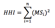 where MS is the market share of each firm, i, operating in a single market. Summing across all squared market shares for all firms results in the measure of concentration in the given market, HHI.
Often, the HHI is used as a measure of competition, with 10,000 equaling perfect monopoly (100^2) and 0.0 equaling perfect competition. As such, we can see that the U.S. men’s footwear industry in 2017 seems relatively competitive. Yet, to say anything substantive about the men’s U.S. footwear market, we really need a comparison of HHI scores for this market over time. This is where the second command comes in.
Let’s return to our men’s U.S. footwear example to see how the function works in practice. First, we need to calculate the HHI scores for each year in the data file (2012-2017), and store those as objects to make a data frame of HHI scores corresponding to individual years. Then, we simply call the plot_hhi command and generate a simple, pleasing plot of HHI scores over time. This will give us a much better sense of how our 2017 HHI score above compares with other years in this market. See the code below, followed by the output.
These lines of code will give us the following plot of HHI scores for each year in the data set.
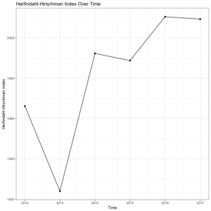
Interestingly, the men’s U.S. footwear industry seems to be getting slightly less competitive (higher HHI scores) from 2012 to 2017, on average. To say anything substantive about this trend, though, would obviously require more sophisticated methods as well as a longer time series. Yet, the value of the hhi package is allowing for quick calculation and visualization of HHI scores over time. You can download the package from CRAN or directly from the package installation context in RStudio. And as always, if you have any questions or find any bugs requiring fixing, please feel free to contact me.
Herfindahl, Orris C. 1950. “Concentration in the steel industry.” Ph.D. dissertation, Columbia University.
Hirschman, Albert O. 1945. “National power and structure of foreign trade.” Berkeley, CA: University of California Press.
Rhoades, Stephen A. 1993. “The herfindahl-hirschman index.” Federal Reserve Bulletin 79: 188.
# First, install the "hhi" package, then load the library
install.packages("hhi")
library(hhi)

# Next, read in data: US Men's Footwear Company Market Shares, 2012-2017
footwear = read.table(".../footwear.txt")

# Now, call the "hhi" command to calculate HHI for 2017
hhi(footwear, "ms.2017") # first the df, then the shares variable in quotes
Often, the HHI is used as a measure of competition, with 10,000 equaling perfect monopoly (100^2) and 0.0 equaling perfect competition. As such, we can see that the U.S. men’s footwear industry in 2017 seems relatively competitive. Yet, to say anything substantive about the men’s U.S. footwear market, we really need a comparison of HHI scores for this market over time. This is where the second command comes in.
Let’s return to our men’s U.S. footwear example to see how the function works in practice. First, we need to calculate the HHI scores for each year in the data file (2012-2017), and store those as objects to make a data frame of HHI scores corresponding to individual years. Then, we simply call the plot_hhi command and generate a simple, pleasing plot of HHI scores over time. This will give us a much better sense of how our 2017 HHI score above compares with other years in this market. See the code below, followed by the output.
# First, calculate and store HHI for each year in the data file (2012-2017)
hhi.12 = hhi(footwear, "ms.2012")
hhi.13 = hhi(footwear, "ms.2013")
hhi.14 = hhi(footwear, "ms.2014")
hhi.15 = hhi(footwear, "ms.2015")
hhi.16 = hhi(footwear, "ms.2016")
hhi.17 = hhi(footwear, "ms.2017")

# Combine and create df for plotting
hhi = rbind(hhi.12, hhi.13, hhi.14, hhi.15, hhi.16, hhi.17)

year = c(2012, 2013, 2014, 2015, 2016, 2017)

hhi.data = data.frame(year, hhi)

# Finally, generate HHI time series plot using the "plot_hhi" command
plot_hhi(hhi.data, "year", "hhi")
These lines of code will give us the following plot of HHI scores for each year in the data set.
Interestingly, the men’s U.S. footwear industry seems to be getting slightly less competitive (higher HHI scores) from 2012 to 2017, on average. To say anything substantive about this trend, though, would obviously require more sophisticated methods as well as a longer time series. Yet, the value of the hhi package is allowing for quick calculation and visualization of HHI scores over time. You can download the package from CRAN or directly from the package installation context in RStudio. And as always, if you have any questions or find any bugs requiring fixing, please feel free to contact me.
Herfindahl, Orris C. 1950. “Concentration in the steel industry.” Ph.D. dissertation, Columbia University.
Hirschman, Albert O. 1945. “National power and structure of foreign trade.” Berkeley, CA: University of California Press.
Rhoades, Stephen A. 1993. “The herfindahl-hirschman index.” Federal Reserve Bulletin 79: 188.
Introducing purging: An R package for addressing mediation effects
A Simple Method for Purging Mediation Effects among Independent Variables
Mediation can occur when one independent variable swamps the effect of another, suggesting high correlation between the two variables. Though there are some great packages for mediation analysis out there, the simple intuition of its need is often ambiguous, especially for younger graduate students. Thus, in this blog post, it is my goal to introduce an intuitive overview of mediation and offer a simple method for “purging” variables of mediation effects for their simultaneous use in multivariate analysis. The purging process detailed in this blog is available in my recently released R package, purging, which is available on CRAN or at my GitHub.
Let’s consider a couple practical examples from “real life” research contexts. First, suppose we are interested in whether committee membership relating to a specific issue domain influences the likelihood of sponsoring related issue-specific legislation. However, in the American context as representational responsibilities permeate legislative behavior, district characteristics in similar employment-related industries likely influence self-selection onto the issue-specific committees in the first place, which we also suggest should influence likelihood of related-issue bill sponsorship. Therefore, in this context, we have a mediation model, where employment/industry (indirect) -> committee membership (direct) -> sponsorship. Thus, we would want to purge committee membership of the effects of employment/industry in the district to observe the “pure” effect of committee membership on the likelihood of related sponsorship. This example is from my paper recently published in American Politics Research.
Or consider a second example in a different realm. Let’s say we had a model where women’s level of labor force participation determines their level of contraceptive use, and that the effect of female labor force participation on fertility is indirect, essentially filtered through its impact on contraceptive use. Once we control for contraceptive use, the direct effect of labor force participation may go away. In other words, the effect of labor force participation on fertility is likely indirect, and filtered through contraceptive use, which means the variables are also highly correlated. This second example was borrowed from Scott Basinger’s and Patrick Shea’s (University of Houston) graduate statistics labs, which originally gave me the idea of expanding this out to develop an R package dedicated to addressing this issue in a variety of contexts and for several functional forms.
These two examples offer simple ways of thinking about mediation effects (e.g., labor force (indirect) -> contraception (direct) -> fertility). If we run into this problem, a simple solution is “purging”. The steps to purge are to, first, regress the direct variable (in the second case, “contraceptive use”) on the indirect variable (in the second case, “labor force participation”). Then, store those residuals, which is the direct effect of contraception after accounting for the indirect effect of labor force participation. Then, we add the stored residuals as their own “purged variable” in the updated specification. Essentially, this purging process allows for a new direct variable that is uncorrelated with the indirect variable. When we do this, we will see that each variable is explaining unique variance in the DV of interest (you can double check this several ways, such as comparing correlation coefficients (which we will do below) or by comparing R^2 across specifications).
An Applied Example
With the intuition behind mediation and the purging solution in mind, let’s walk through a simple example using some fake data. For an example based on the second case described above using real data from the United Nations Human Development Programme, see the code file, purging example.R, at my GitHub repository.
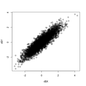
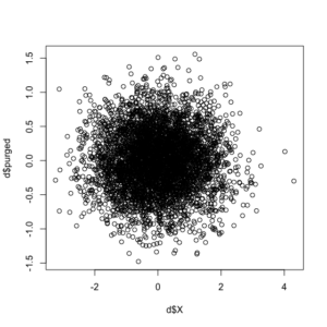
In addition to the correlation coefficient between the two variables being exactly as we specified (0.90), see this positive correlation between the two random variables in the plot below.
Now, with our correlated data created, we can call the “purge.lm” command, given that our data are continuous. Note: the package supports a variety of functional forms for continuous (linear), binary (logit and probit), and event count data (Poisson and negative binomial).
The idea behind the package is to generate the new direct-impact variable to be used in the analysis, purged of the effects of the indirect variable. To do so, simply input the name of the data frame first, followed by the name of the direct variable in quotes, and then the indirect variable also in quotes in the function. Calling the function will generate a new object (i.e., the direct variable), which can then be added to a data frame using the $ operator, with the following line of code:
Note the correlation between the original indirect (X) variable and the new direct (Y) variable, purged of the effects of X, is -9.211365e-17, or essentially non-existent. For additional corroboration, let’s see the updated correlation plot between the X and purged-Y variables.
The purge command did as expected, with the correlation between the two variables essentially gone. You can download the package and documentation at CRAN. If you have any questions or find any bugs requiring fixing, please feel free to contact me. As this procedure was first developed and implemented (using the binary/logit iteration discussed above in the first example) in a now-published paper, please cite use of the package as: Waggoner, Philip D. 2018. “Do Constituents Influence Issue-Specific Bill Sponsorship?” American Politics Research, <https://doi.org/10.1177/1532673X18759644>
As a final note, once the intuition is mastered, be sure to check out the great work on mediation from many folks, including Kosuke Imai (Princeton), Luke Keele (Georgetown), and several others. See Imai’s mediation site as a sound starting place with code, papers, and more.
Thanks and enjoy!
Mediation can occur when one independent variable swamps the effect of another, suggesting high correlation between the two variables. Though there are some great packages for mediation analysis out there, the simple intuition of its need is often ambiguous, especially for younger graduate students. Thus, in this blog post, it is my goal to introduce an intuitive overview of mediation and offer a simple method for “purging” variables of mediation effects for their simultaneous use in multivariate analysis. The purging process detailed in this blog is available in my recently released R package, purging, which is available on CRAN or at my GitHub.
Let’s consider a couple practical examples from “real life” research contexts. First, suppose we are interested in whether committee membership relating to a specific issue domain influences the likelihood of sponsoring related issue-specific legislation. However, in the American context as representational responsibilities permeate legislative behavior, district characteristics in similar employment-related industries likely influence self-selection onto the issue-specific committees in the first place, which we also suggest should influence likelihood of related-issue bill sponsorship. Therefore, in this context, we have a mediation model, where employment/industry (indirect) -> committee membership (direct) -> sponsorship. Thus, we would want to purge committee membership of the effects of employment/industry in the district to observe the “pure” effect of committee membership on the likelihood of related sponsorship. This example is from my paper recently published in American Politics Research.
Or consider a second example in a different realm. Let’s say we had a model where women’s level of labor force participation determines their level of contraceptive use, and that the effect of female labor force participation on fertility is indirect, essentially filtered through its impact on contraceptive use. Once we control for contraceptive use, the direct effect of labor force participation may go away. In other words, the effect of labor force participation on fertility is likely indirect, and filtered through contraceptive use, which means the variables are also highly correlated. This second example was borrowed from Scott Basinger’s and Patrick Shea’s (University of Houston) graduate statistics labs, which originally gave me the idea of expanding this out to develop an R package dedicated to addressing this issue in a variety of contexts and for several functional forms.
These two examples offer simple ways of thinking about mediation effects (e.g., labor force (indirect) -> contraception (direct) -> fertility). If we run into this problem, a simple solution is “purging”. The steps to purge are to, first, regress the direct variable (in the second case, “contraceptive use”) on the indirect variable (in the second case, “labor force participation”). Then, store those residuals, which is the direct effect of contraception after accounting for the indirect effect of labor force participation. Then, we add the stored residuals as their own “purged variable” in the updated specification. Essentially, this purging process allows for a new direct variable that is uncorrelated with the indirect variable. When we do this, we will see that each variable is explaining unique variance in the DV of interest (you can double check this several ways, such as comparing correlation coefficients (which we will do below) or by comparing R^2 across specifications).
An Applied Example
With the intuition behind mediation and the purging solution in mind, let’s walk through a simple example using some fake data. For an example based on the second case described above using real data from the United Nations Human Development Programme, see the code file, purging example.R, at my GitHub repository.
# First, install the MASS package for the "mvrnorm" function
install.packages("MASS")
library(MASS)
# Second, install the purging package directly from CRAN for the "purge.lm" function
install.packages("purging")
library(purging)

# Set some paramters to guide our simulation
n = 5000
rho = 0.9

# Create some fake data
d = mvrnorm(n = n, mu = c(0, 0), Sigma = matrix(c(1, rho, rho, 1), nrow = 2), empirical = TRUE)

# Store each correlated variable as its own object
X = d[, 1]
Y = d[, 2]

# Create a dataframe of your two variables
d = data.frame(X, Y)

# Verify the correlation between these two normally distributed variables is what we set (rho = 0.9)
cor(d$X, d$Y)
plot(d$X, d$Y)
In addition to the correlation coefficient between the two variables being exactly as we specified (0.90), see this positive correlation between the two random variables in the plot below.
Now, with our correlated data created, we can call the “purge.lm” command, given that our data are continuous. Note: the package supports a variety of functional forms for continuous (linear), binary (logit and probit), and event count data (Poisson and negative binomial).
The idea behind the package is to generate the new direct-impact variable to be used in the analysis, purged of the effects of the indirect variable. To do so, simply input the name of the data frame first, followed by the name of the direct variable in quotes, and then the indirect variable also in quotes in the function. Calling the function will generate a new object (i.e., the direct variable), which can then be added to a data frame using the $ operator, with the following line of code:
df$purged.var <- purged.varLet’s now see the purge command in action using our fake data.
# Purge the "direct" variable, Y, of the mediation effects of X
# (direct/indirect selection will depend on your model specification)
purge.lm(d, "Y", "X") # df, "direct", "indirect"

# You will get an automatic suggestion message to store the values in the df
purged = purge.lm(d, "Y", "X") # Store as its own object
d$purged = purged # Attach to df

# Finally, check the correlation and the plot to see the effects purged from the original "Y" (direct) variable
cor(d$X, d$purged)
plot(d$X, d$purged)
Note the correlation between the original indirect (X) variable and the new direct (Y) variable, purged of the effects of X, is -9.211365e-17, or essentially non-existent. For additional corroboration, let’s see the updated correlation plot between the X and purged-Y variables.
The purge command did as expected, with the correlation between the two variables essentially gone. You can download the package and documentation at CRAN. If you have any questions or find any bugs requiring fixing, please feel free to contact me. As this procedure was first developed and implemented (using the binary/logit iteration discussed above in the first example) in a now-published paper, please cite use of the package as: Waggoner, Philip D. 2018. “Do Constituents Influence Issue-Specific Bill Sponsorship?” American Politics Research, <https://doi.org/10.1177/1532673X18759644>
As a final note, once the intuition is mastered, be sure to check out the great work on mediation from many folks, including Kosuke Imai (Princeton), Luke Keele (Georgetown), and several others. See Imai’s mediation site as a sound starting place with code, papers, and more.
Thanks and enjoy!
Discriminant Analysis: Statistics All The Way
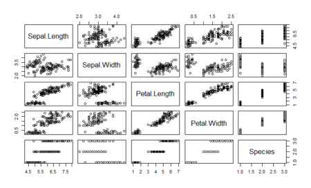
Discriminant analysis is used when the variable to be predicted is categorical in nature. This analysis requires that the way to define data points to the respective categories is known which makes it different from cluster analysis where the classification criteria is not know. It works by calculating a score based on all the predictor variables and based on the values of the score, a corresponding class is selected. Hence, the name discriminant analysis which, in simple terms, discriminates data points and classifies them into classes or categories based on analysis of the predictor variables. This article delves into the linear discriminant analysis function in R and delivers in-depth explanation of the process and concepts. Before we move further, let us look at the assumptions of discriminant analysis which are quite similar to MANOVA.
(x−μ1)TΣ1−1(x−μ1)+ln|Σ1|−(x−μ2)TΣ2−1(x−μ2)−ln|Σ2|T
As we can see, one of the classes is completely separate while the other two are somewhat overlapping. However, LDA is still able to distinguish between the two. A better version of using lda is lda() with CV. This can be done by passing the CV=TRUE in the lda function.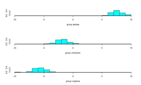
The data points are almost completely separated by the first linear discriminant and that is why we see the three classes in different ranges of values. To further our understanding, we also see the second linear discriminant.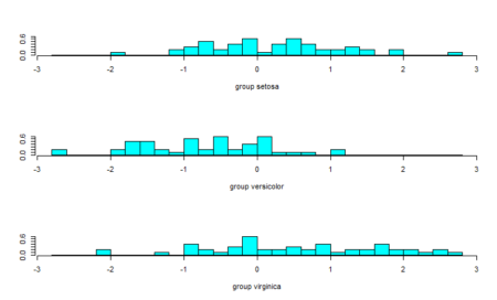
From the plot of the second linear discriminant, we see that we can hardly differentiate between the three groups hence the proportion of trace values.
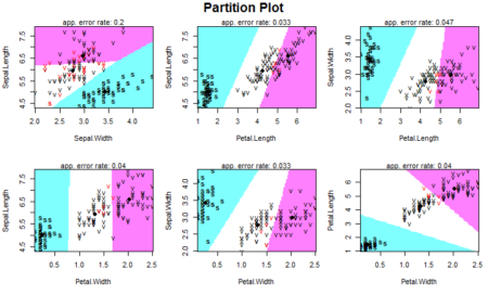
Our data has four features so we have 4C2 =6 combinations to classify our data. The plot show how different classes are defined based on the two features on x-axis and y-axis. As a summary, it is important to know that one should look at the data first to know whether the data seems to be linearly separable (or quadratically separable in case of qda) before selecting the technique. Since LDA makes some assumptions about the data, we also need to preprocess the data and perform univariate analysis to see if the normality assumption holds for each class of the data. In the absence of normality, that is, in case there is a violation of the normality condition, one can still proceed with LDA or QDA but the results will not be appropriate and will lack in accuracy. We also need to analyze whether the features are related to each other and some of them need to be omitted from our analysis. The rest is up to the lda() function to calculate and make predictions on. Here is the entire code used in this article:
- Since we are dealing with multiple features, one of the first assumptions that the technique makes is the assumption of multivariate normality that means the features are normally distributed when separated for each class. This also implies that the technique is susceptible to possible outliers and is also sensitive to the group sizes. If there is an imbalance between the group sizes and one of the groups is too small or too large, the technique suffers when classifying data points into that ‘outlier’ class
(x−μ1)TΣ1−1(x−μ1)+ln|Σ1|−(x−μ2)TΣ2−1(x−μ2)−ln|Σ2|T
Where (μ1,Σ1) and(μ2, Σ2) are the respective means and variances of x for class 1 and class 2. We sometimes simplify our calculations by assuming equal variances of the two classes to get a simplified version
w.x>c where c is the threshold and w is the weight combined with x.
Let’s understand Fisher’s LDA which is one of the most popular variants of LDA
Fisher’s Linear Discriminant analysis – How and when to use it?
Fisher’s linear discriminant finds out a linear combination of features that can be used to discriminate between the target variable classes. In Fisher’s LDA, we take the separation by the ratio of the variance between the classes to the variance within the classes. To understand it in a different way, it is the interclass variance to intraclass variance ratio
S= 𝛔2between/𝛔2within = (w⋅(μ2−μ1))2/ wT(Σ1+Σ2)w
Fisher’s LDA maximizes this ratio and has a lot of applications. One of the recent applications involve classification of speech and audio. Other past usages include face recognition where Fisher’s LDA is used to create Fisher’s Faces and combined with PCA technique to get eigenfaces. Fisher’s LDA also finds usages in earth science, biomedical science, bankruptcy problems and finance along with in marketing. That’s all on the theoretical aspect of LDA. Let’s understand using an example in R.
LDA Classification example in R
R has a MASS package which has the lda() function. For dataset, we will use the iris dataset and try to classify the classes.
#Load the library containing lda() function
library(MASS)
#Store the dataset
dataset=iris

Before running the lda() function, let’s start with the help documentation of lda()
#Help Documentation
?lda
The description for lda() is minimalistic and simple. We are interested in the details section of the documentation which describes the process which the function uses. As the documentation mentions – the lda() function also tries to detect if the within-class covariance matrix is singular. We can also define a tolerance such that if any variable has within-group variance less than tol^2 it will stop and report the variable as a constant.
Another possible adjustment is the prior probabilities. The prior parameter in lda() function is used to specify the prior probabilities. If not specified, the function calculates the prior probabilities to be the same as the distribution of classes in the data. These prior probabilities also affect the rotation of the linear discriminants.
Let us proceed with performing linear discriminant analysis over the iris dataset.
#Perform LDA over the data
lda_iris=lda(Species~.,data=dataset)
#Prior Probabilities and coefficients of Linear discriminants
lda_iris

Call:
lda(Species ~ ., data = dataset)

Prior probabilities of groups:
        setosa      versicolor      virginica
    0.3333333   0.3333333   0.3333333

Group means:
                Sepal.Length        Sepal.Width         Petal.Length        Petal.Width
setosa              5.006               3.428               1.462               0.246
versicolor          5.936               2.770               4.260               1.326
virginica           6.588               2.974               5.552               2.026

Coefficients of linear discriminants:
                            LD1             LD2
Sepal.Length        0.8293776   0.02410215
Sepal.Width         1.5344731   2.16452123
Petal.Length        -2.2012117  -0.93192121
Petal.Width         -2.8104603      2.83918785

Proportion of trace:
        LD1         LD2
0.9912  0.0088


#Check the accuracy of our analysis
Predictions=predict(lda_iris,dataset)
table(Predictions$class, dataset$Species)
                setosa      versicolor  virginica
  setosa            50              0           0
  versicolor        0           48          1
  virginica         0           2           49
With LDA, we are able to classify all but 3 data points correctly in iris dataset. This is probably because the iris data is linearly separable. How do we know whether a data is linearly separable or not? We use the pairs function to see the scatter plots of data and see if they are separable
#Check how easily we can linearly separate the iris dataset
pairs(dataset)
As we can see, one of the classes is completely separate while the other two are somewhat overlapping. However, LDA is still able to distinguish between the two. A better version of using lda is lda() with CV. This can be done by passing the CV=TRUE in the lda function.
#LDA with CV
lda_cv_iris=lda(Species~.,data=dataset,CV=TRUE)

#The predictions are already generated in lda_cv_iris
table(lda_cv_iris$class, dataset$Species)
I didn’t generate the summary for the model as it will also produce all the predictions. As we already know from the summary of lda_iris, the function first calculates the prior probabilities of the classes in the dataset unless provided specifically. The iris dataset had 50 data points for each class hence the prior probabilities are calculated to be 0.33 each. It then makes the necessary calculations which involves means of each class and overall variance and gets the linear discriminant. The function also scales the value of the linear discriminants so that the mean is zero and variance is one. The final value, proportion of trace that we get is the percentage separation that each of the discriminant achieves. Thus, the first linear discriminant is enough and achieves about 99% of the separation.
As a final step, we will plot the linear discriminants and visually see the difference in distinguishing ability. The ldahist() function helps make the separator plot. For the data into the ldahist() function, we can use the x[,1] for the first linear discriminant and x[,2] for the second linear discriminant and so on
#Plot the predictions - first linear discriminant
ldahist(data = Predictions$x[,1], g=Species)
The data points are almost completely separated by the first linear discriminant and that is why we see the three classes in different ranges of values. To further our understanding, we also see the second linear discriminant.
#Plot the predictions - second linear discriminant
ldahist(data = Predictions$x[,2], g=Species)
From the plot of the second linear discriminant, we see that we can hardly differentiate between the three groups hence the proportion of trace values.
Everything is not linear – quadratic discriminant analysis
MASS package also contains the qda() function which stands for quadratic discriminant analysis. The idea is simple – if the data can be discriminated using a quadratic function, we can use qda() instead of lda(). The rest of the nuances are the same for qda() as were in lda()
#QDA
qda_iris=qda(Species~.,data=dataset)
qda_iris


Call:
qda(Species ~ ., data = dataset)

Prior probabilities of groups:
            setosa      versicolor      virginica
        0.3333333   0.3333333   0.3333333

Group means:
                Sepal.Length        Sepal.Width         Petal.Length        Petal.Width
setosa              5.006               3.428               1.462               0.246
versicolor          5.936               2.770               4.260               1.326
virginica           6.588               2.974               5.552               2.026

#Check the accuracy of our analysis of qda
Predictions_qda=predict(qda_iris,dataset)
table(Predictions_qda$class, dataset$Species)
                setosa      versicolor  virginica
  setosa            50              0           0
  versicolor        0           48          1
  virginica         0           2           49
Since the data has a linear relation, the qda function also applies the same statistics and returns similar results.
Conclusion: Evaluating LDA and QDA
Even though LDA is a tough problem to understand, its implementation in R is simple. As a final step, we will look into another package- the klaR package which helps to create an exploratory graph for LDA or QDA.
The package contains the partimat() function which takes a similar input as the lda() function but returns a plot instead of the model. The function stands for partition matrix and plots the ability of the features to partition the target class taking combinations of two at a time.
#Using the klarR package
# install.packages("klaR")
library(klaR)
partimat(Species~.,data=dataset,method="lda")
Our data has four features so we have 4C2 =6 combinations to classify our data. The plot show how different classes are defined based on the two features on x-axis and y-axis. As a summary, it is important to know that one should look at the data first to know whether the data seems to be linearly separable (or quadratically separable in case of qda) before selecting the technique. Since LDA makes some assumptions about the data, we also need to preprocess the data and perform univariate analysis to see if the normality assumption holds for each class of the data. In the absence of normality, that is, in case there is a violation of the normality condition, one can still proceed with LDA or QDA but the results will not be appropriate and will lack in accuracy. We also need to analyze whether the features are related to each other and some of them need to be omitted from our analysis. The rest is up to the lda() function to calculate and make predictions on. Here is the entire code used in this article:
#Load the library containing lda() function
library(MASS)
#Store the dataset
dataset=iris

#Help Documentation
?lda

#Perform LDA over the data
lda_iris=lda(Species~.,data=dataset)
#Prior Probabilities and coefficients of Linear discriminants
lda_iris

#Check the accuracy of our analysis
Predictions=predict(lda_iris,dataset)
table(Predictions$class, dataset$Species)

#Check how easily we can linearly separate the iris dataset
pairs(dataset)

#LDA with CV
lda_cv_iris=lda(Species~.,data=dataset,CV=TRUE)

#The predictions are already generated in lda_cv_iris
table(lda_cv_iris$class, dataset$Species)

#Plot the predictions - first linear discriminant
ldahist(data = Predictions$x[,1], g=Species)

#Plot the predictions - second linear discriminant
ldahist(data = Predictions$x[,2], g=Species)

#QDA
qda_iris=qda(Species~.,data=dataset)
qda_iris

#Check the accuracy of our analysis of qda
Predictions_qda=predict(qda_iris,dataset)
table(Predictions_qda$class, dataset$Species)

#Using the klarR packagew
# install.packages("klaR")
library(klaR)
partimat(Species~.,data=dataset,method="lda")
Author Bio:
This article was contributed by Perceptive Analytics. Madhur Modi, Chaitanya Sagar, Jyothirmayee Thondamallu and Saneesh Veetil contributed to this article.
Perceptive Analytics provides data analytics, data visualization, business intelligence and reporting services to e-commerce, retail, healthcare and pharmaceutical industries. Our client roster includes Fortune 500 and NYSE listed companies in the USA and India.
Steps to Perform Survival Analysis in R
Another way of analysis?
When there are so many tools and techniques of prediction modelling, why do we have another field known as survival analysis? As one of the most popular branch of statistics, Survival analysis is a way of prediction at various points in time. This is to say, while other prediction models make predictions of whether an event will occur, survival analysis predicts whether the event will occur at a specified time. Thus, it requires a time component for prediction and correspondingly, predicts the time when an event will happen. This helps one in understanding the expected duration of time when events occur and provide much more useful information. One can think of natural areas of application of survival analysis which include biological sciences where one can predict the time for bacteria or other cellular organisms to multiple to a particular size or expected time of decay of atoms. Some interesting applications include prediction of the expected time when a machine will break down and maintenance will be requiredHow hard does it get..
It is not easy to apply the concepts of survival analysis right off the bat. One needs to understand the ways it can be used first. This includes Kaplan-Meier Curves, creating the survival function through tools such as survival trees or survival forests and log-rank test.
Let’s go through each of them one by one in R. We will use the survival package in R as a starting example. The survival package has the surv() function that is the center of survival analysis.
# install.packages("survival")
# Loading the package
library("survival")
The package contains a sample dataset for demonstration purposes. The dataset is pbc which contains a 10 year study of 424 patients having Primary Biliary Cirrhosis (pbc) when treated in Mayo clinic. A point to note here from the dataset description is that out of 424 patients, 312 participated in the trial of drug D-penicillamine and the rest 112 consented to have their basic measurements recorded and followed for survival but did not participate in the trial. 6 of these 112 cases were lost.
We are particularly interested in ‘time’ and ‘status’ features in the dataset. Time represents the number of days after registration and final status (which can be censored, liver transplant or dead). Since it is survival, we will consider the status as dead or not-dead (transplant or censored). Further details about the dataset can be read from the command:
#Dataset description
?pbc
We start with a direct application of the Surv() function and pass it to the survfit() function. The Surv() function will take the time and status parameters and create a survival object out of it. The survfit() function takes a survival object (the one which Surv() produces) and creates the survival curves.
#Fitting the survival model
survival_func=survfit(Surv(pbc$time,pbc$status == 2)~1)
survival_func

Call: survfit(formula = Surv(pbc$time, pbc$status == 2) ~ 1)

        n   events      median  0.95LCL     0.95UCL
        418         161         3395        3090        3853
The function gives us the number of values, the number of positives in status, the median time and 95% confidence interval values. The model can also be plotted.
#Plot the survival model
plot(survival_func)
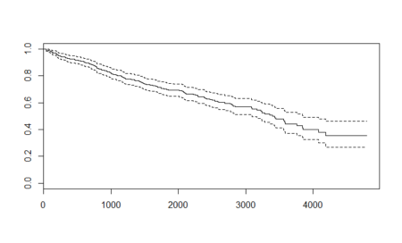
As expected, the plot shows us the decreasing probabilities for survival as time passes. The dashed lines are the upper and lower confidence intervals. In the survfit() function here, we passed the formula as ~ 1 which indicates that we are asking the function to fit the model solely on the basis of survival object and thus have an intercept. The output along with the confidence intervals are actually Kaplan-Meier estimates. This estimate is prominent in medical research survival analysis. The Kaplan – Meier estimates are based on the number of patients (each patient as a row of data) from the total number who survive for a certain time after treatment. (which is the event). We can represent the Kaplan – Meier function by the formula:
Ŝ(t)=∏(1-di/ni) for all i where ti≤t
Here, di the number of events and ni is the total number of people at risk at time ti
What to make of the graph?
Unlike other machine learning techniques where one uses test samples and makes predictions over them, the survival analysis curve is a self – explanatory curve. From the curve, we see that the possibility of surviving about 1000 days after treatment is roughly 0.8 or 80%. We can similarly define probability of survival for different number of days after treatment. At the same time, we also have the confidence interval ranges which show the margin of expected error. For example, in case of surviving 1000 days example, the upper confidence interval reaches about 0.85 or 85% and goes down to about 0.75 or 75%. Post the data range, which is 10 years or about 3500 days, the probability calculations are very erratic and vague and should not be taken up. For example, if one wants to know the probability of surviving 4500 days after treatment, then though the Kaplan – Meier graph above shows a range between 0.25 to 0.55 which is itself a large value to accommodate the lack of data, the data is still not sufficient enough and a better data should be used to make such an estimate.Alternative models: Cox Proportional Hazard model
The survival package also contains a cox proportional hazard function coxph() and use other features in the data to make a better survival model. Though the data has untreated missing values, I am skipping the data processing and fitting the model directly. In practice, however, one needs to study the data and look at ways to process the data appropriately so that the best possible models are fitted. As the intention of this article is to get the readers acquainted with the function rather than processing, applying the function is the shortcut step which I am taking.
# Fit Cox Model
Cox_model = coxph(Surv(pbc$time,pbc$status==2) ~.,data=pbc)
summary(Cox_model)

Call:
coxph(formula = Surv(pbc$time, pbc$status == 2) ~ ., data = pbc)

  n= 276, number of events= 111
   (142 observations deleted due to missingness)

                coef    exp(coef)       se(coef)        z   Pr(>|z|)
id              -2.729e-03      9.973e-01   1.462e-03   -1.866  0.06203 .
trt             -1.116e-01      8.944e-01   2.156e-01   -0.518  0.60476
age         3.191e-02   1.032e+00   1.200e-02   2.659   0.00784 **
sexf            -3.822e-01      6.824e-01   3.074e-01   -1.243  0.21378
ascites     6.321e-02   1.065e+00   3.874e-01   0.163   0.87038
hepato      6.257e-02   1.065e+00   2.521e-01   0.248   0.80397
spiders     7.594e-02   1.079e+00   2.448e-01   0.310   0.75635
edema       8.860e-01   2.425e+00   4.078e-01   2.173   0.02980 *
bili            8.038e-02   1.084e+00   2.539e-02   3.166   0.00155 **
chol        5.151e-04   1.001e+00   4.409e-04   1.168   0.24272
albumin     -8.511e-01      4.270e-01   3.114e-01   -2.733  0.00627 **
copper      2.612e-03   1.003e+00   1.148e-03   2.275   0.02290 *
alk.phos    -2.623e-05      1.000e+00   4.206e-05   -0.624  0.53288
ast         4.239e-03   1.004e+00   1.941e-03   2.184   0.02894 *
trig            -1.228e-03      9.988e-01   1.334e-03   -0.920  0.35741
platelet    7.272e-04   1.001e+00   1.177e-03   0.618   0.53660
protime     1.895e-01   1.209e+00   1.128e-01   1.680   0.09289 .
stage       4.468e-01   1.563e+00   1.784e-01   2.504   0.01226 *
---
Signif. codes:  0 ‘***’ 0.001 ‘**’ 0.01 ‘*’ 0.05 ‘.’ 0.1 ‘ ’ 1

                exp(coef)   exp(-coef)  lower .95   upper .95
id              0.9973      1.0027      0.9944      1.000
trt             0.8944      1.1181      0.5862      1.365
age             1.0324      0.9686      1.0084      1.057
sexf            0.6824      1.4655      0.3736      1.246
ascites         1.0653      0.9387      0.4985      2.276
hepato          1.0646      0.9393      0.6495      1.745
spiders         1.0789      0.9269      0.6678      1.743
edema           2.4253      0.4123      1.0907      5.393
bili            1.0837      0.9228      1.0311      1.139
chol            1.0005      0.9995      0.9997      1.001
albumin     0.4270      2.3422      0.2319      0.786
copper          1.0026      0.9974      1.0004      1.005
alk.phos        1.0000      1.0000      0.9999      1.000
ast             1.0042      0.9958      1.0004      1.008
trig            0.9988      1.0012      0.9962      1.001
platelet        1.0007      0.9993      0.9984      1.003
protime         1.2086      0.8274      0.9690      1.508
stage           1.5634      0.6397      1.1020      2.218

Concordance= 0.849  (se = 0.031 )
Rsquare= 0.462   (max possible= 0.981 )
Likelihood ratio test= 171.3  on 18 df,   p=0
Wald test            = 172.5  on 18 df,   p=0
Score (logrank) test = 286.1  on 18 df,   p=0
The Cox model output is similar to how a linear regression output comes up. The R2 is only 46% which is not high and we don’t have any feature which is highly significant. The top important features appear to be age, bilirubin (bili) and albumin. Let’s see how the plot looks like.
#Create a survival curve from the cox model
Cox_curve <- survfit(Cox_model)
plot(Cox_curve)
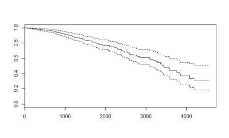
With more data, we get a different plot and this one is more volatile. Compared to the Kaplan – Meier curve, the cox-plot curve is higher for the initial values and lower for the higher values. The major reason for this difference is the inclusion of variables in cox-model. The plots are made by similar functions and can be interpreted the same way as the Kaplan – Meier curve.
Going traditional : Using survival forests
Random forests can also be used for survival analysis and the ranger package in R provides the functionality. However, the ranger function cannot handle the missing values so I will use a smaller data with all rows having NA values dropped. This will reduce my data to only 276 observations.
#Using the Ranger package for survival analysis
Install.packages("ranger")
library(ranger)

#Drop rows with NA values
pbc_nadrop=pbc[complete.cases(pbc), ]
#Fitting the random forest
ranger_model <- ranger(Surv(pbc_nadrop$time,pbc_nadrop$status==2) ~.,data=pbc_nadrop,num.trees = 500, importance = "permutation",seed = 1)

#Plot the death times
plot(ranger_model$unique.death.times,ranger_model$survival[1,], type = "l", ylim = c(0,1),)
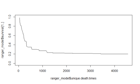
Let’s look at the variable importance plot which the random forest model calculates.
#Get the variable importance
data.frame(sort(ranger_model$variable.importance,decreasing = TRUE))
sort.ranger_model.variable.importance..decreasing...TRUE.

bili                                                    0.0762338981
copper                                                  0.0202733989
albumin                                                 0.0165070226
age                                                     0.0130134413
edema                                                   0.0122113704
ascites                                                 0.0115315711
chol                                                    0.0092889960
protime                                                 0.0060215073
id                                                      0.0055867915
ast                                                     0.0049932803
stage                                                   0.0030225398
hepato                                                  0.0029290675
trig                                                    0.0028869184
platelet                                                0.0012958105
sex                                                     0.0010639806
spiders                                                 0.0005210531
alk.phos                                                0.0003291581
trt                                                     -0.0002020952
These numbers may be different for different runs. In my example, we see that bilirubin is the most important feature.
Lessons learned: Conclusion
Though the input data for Survival package’s Kaplan – Meier estimate, Cox Model and ranger model are all different, we will compare the methodologies by plotting them on the same graph using ggplot.#Comparing models
library(ggplot2)
#Kaplan-Meier curve dataframe
#Add a row of model name
km <- rep("Kaplan Meier", length(survival_func$time))
#Create a dataframe
km_df <- data.frame(survival_func$time,survival_func$surv,km)
#Rename the columns so they are same for all dataframes
names(km_df) <- c("Time","Surv","Model")
#Cox model curve dataframe
#Add a row of model name
cox <- rep("Cox",length(Cox_curve$time))
#Create a dataframe
cox_df <- data.frame(Cox_curve$time,Cox_curve$surv,cox)
#Rename the columns so they are same for all dataframes
names(cox_df) <- c("Time","Surv","Model")
#Dataframe for ranger
#Add a row of model name
rf <- rep("Survival Forest",length(ranger_model$unique.death.times))
#Create a dataframe
rf_df <- data.frame(ranger_model$unique.death.times,sapply(data.frame(ranger_model$survival),mean),rf)
#Rename the columns so they are same for all dataframes
names(rf_df) <- c("Time","Surv","Model")
#Combine the results
plot_combo <- rbind(km_df,cox_df,rf_df)
#Make a ggplot
plot_gg <- ggplot(plot_combo, aes(x = Time, y = Surv, color = Model))
plot_gg + geom_line() + ggtitle("Comparison of Survival Curves")
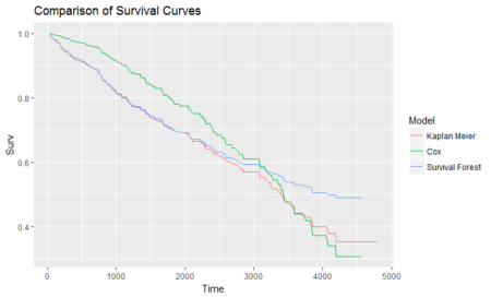
We see here that the Cox model is the most volatile with the most data and features. It is higher for lower values and drops down sharply when the time increases. The survival forest is of the lowest range and resembles Kaplan-Meier curve. The difference might be because of Survival forest having less rows. The essence of the plots is that there can be different approaches to the same concept of survival analysis and one may choose the technique based on one’s comfort and situation. A better data with processed data points and treated missing values might fetch us a better R2 and more stable curves. At the same time, they will help better in finding time to event cases such as knowing the time when a promotion’s effect dies down, knowing when tumors will develop and become significant and lots of other applications with a significant chunk of them being from medical science. Survival, as the name suggests, relates to surviving objects and is thus related to event occurrence in a completely different way than machine learning. It is important to know this technique to know more and more ways data can help us in solving problems, with time involved in this particular case. Hope this article serves the purpose of giving a glimpse of survival analysis and the feature rich packages available in R.
Here is the complete code for the article:
# install.packages("survival")
# Loading the package
library("survival")
#Dataset description
?pbc
#Fitting the survival model
survival_func=survfit(Surv(pbc$time,pbc$status == 2)~1)
survival_func
#Plot the survival model
plot(survival_func)
# Fit Cox Model
Cox_model = coxph(Surv(pbc$time,pbc$status==2) ~.,data=pbc)
summary(Cox_model)
#Create a survival curve from the cox model
Cox_curve <- survfit(Cox_model)
plot(Cox_curve)
#Using the Ranger package for survival analysis
#install.packages("ranger")
library(ranger)
#Drop rows with NA values
pbc_nadrop=pbc[complete.cases(pbc), ]
#Fitting the random forest
ranger_model <- ranger(Surv(pbc_nadrop$time,pbc_nadrop$status==2) ~.,data=pbc_nadrop,num.trees = 500, importance = "permutation",seed = 1)
#Plot the death times
plot(ranger_model$unique.death.times,ranger_model$survival[1,], type = "l", ylim = c(0,1),)
#Get the variable importance
data.frame(sort(ranger_model$variable.importance,decreasing = TRUE))
#Comparing models
library(ggplot2)

#Kaplan-Meier curve dataframe
#Add a row of model name
km <- rep("Kaplan Meier", length(survival_func$time))
#Create a dataframe
km_df <- data.frame(survival_func$time,survival_func$surv,km)
#Rename the columns so they are same for all dataframes
names(km_df) <- c("Time","Surv","Model")

#Cox model curve dataframe
#Add a row of model name
cox <- rep("Cox",length(Cox_curve$time))
#Create a dataframe
cox_df <- data.frame(Cox_curve$time,Cox_curve$surv,cox)
#Rename the columns so they are same for all dataframes
names(cox_df) <- c("Time","Surv","Model")

#Dataframe for ranger
#Add a row of model name
rf <- rep("Survival Forest",length(ranger_model$unique.death.times))
#Create a dataframe
rf_df <- data.frame(ranger_model$unique.death.times,sapply(data.frame(ranger_model$survival),mean),rf)
#Rename the columns so they are same for all dataframes
names(rf_df) <- c("Time","Surv","Model")

#Combine the results
plot_combo <- rbind(km_df,cox_df,rf_df)

#Make a ggplot
plot_gg <- ggplot(plot_combo, aes(x = Time, y = Surv, color = Model))
plot_gg + geom_line() + ggtitle("Comparison of Survival Curves")
Author Bio:
This article was contributed by Perceptive Analytics. Madhur Modi, Chaitanya Sagar, Vishnu Reddy and Saneesh Veetil contributed to this article.Perceptive Analytics provides data analytics, data visualization, business intelligence and reporting services to e-commerce, retail, healthcare and pharmaceutical industries. Our client roster includes Fortune 500 and NYSE listed companies in the USA and India.
Whys and Hows of Apply Family of Functions in R
Introduction to Looping system
Imagine you were to perform a simple task, let’s say calculating sum of columns for 3X3 matrix, what do you think is the best way? Calculating it directly using traditional methods such as calculator or even pen and paper doesn’t sound like a bad approach. A lot of us may prefer to just calculate it manually instead of writing an entire piece of code for such a small dataset.Now, if the dataset is 10X10 matrix, would you do the same? Not sure.
Now, if the dataset is further bigger, let’s say 100X100 matrix or 1000X1000 matrix or 5000X5000 matrix, would you even think of doing it manually? I won’t.
But, let’s not worry ourselves with this task because it is not as big a task as it may look at prima facie. There’s a concept called ‘looping’ which comes to our rescue in such situations. I’m sure whosoever has ever worked on any programming language, they must have encountered loops and looping system. It is one of the most useful concepts in any programming language. ‘Looping system’ is nothing but an iterative system that performs a specific task repeatedly until given conditions are met or it is forced to break. Looping system comes in handy when we have to carry a task iteratively; we may or may not know before-hand how many iterations to be carried out. Instead of writing the same piece of code tens or hundreds or thousands of times, we write a small piece of code using loops and it does the entire task for us.
There are majorly two loops which are used extensively in programming – for loop and while loop. In the case of ‘for loop’ we know before hand as to how many times we want the loop to run or we know before-hand the number of iterations that should be carried out. Let’s take a very simple example of printing number 1 to 10. One way could be we write the code of printing every number from 1 to 10; while, the other and smart way would be to write a two-line code that will do the work for us.
for (i in 1:10) {
  print(i)
}
The above code should print values from 1 to 10 for us.
> for (i in 1:10) {
+   print(i)
+ }
[1] 1
[1] 2
[1] 3
[1] 4
[1] 5
[1] 6
[1] 7
[1] 8
[1] 9
[1] 10
The other very powerful loop is ‘while’ loop. In while loop, we don’t know before-hand as to how many iterations should the loop perform. It works till a certain condition is being met, as soon as the condition is violated the loop breaks.
i = 1
while (i < 10) {
  print(i)
  i = i+1
}
In the above code, we don’t know how many iterations are there, we just know that the loop should work until the value of ‘i’ is less than 10 and it does the same.
> i = 1
> while (i < 10) {
+   print(i)
+   i = i+1
+ }
[1] 1
[1] 2
[1] 3
[1] 4
[1] 5
[1] 6
[1] 7
[1] 8
[1] 9
Using very basic examples, we have seen how powerful these loops can be. However, there is one disadvantage of using these loops in R language – they make our code run slow. The number of computations that needs to be carried increases and this increases the time that system takes to execute the code. But we need not worry about this limitation as R offers a very good alternative, vectorization, to using these loops in lot of conditions. Vectorization, as the name suggests, is an operation of converting scalars or plain numbers in to single operation on vectors or matrices. A lot of functions that are performed by loops can be performed through vectorization. Moreover, vectorization makes calculation and running of processes faster because they convert the code into lower language such as C, C++ which further contains loops to execute the operation. User need not worry about these aspects of vectorization and can just do fine with direct functions.
Based on the concept of vectorization is a family of functions in R called ‘apply’ family function. It is a part of base R package. There are multiple functions in the apply family. We will go through them one by one and check their implementation, alongside, in R. The functions in apply family are apply, sapply, lapply, mapply, rapply, tapply and vapply. Their usage depends on the kind of input data we have, kind of output we want to see and the kind of operations we want to perform on data. Let’s go through some of these functions and implement toy examples using them.
Apply Function
Apply function is the most commonly used function in apply family. It works on arrays or matrices. The syntax of apply function is follows:Apply(x, margin, function, ….)Where,
- X refers to an array or matrix on which operation is to be performed
- Margin refers to how the function is to be applied; margin =1 means function is to be applied on rows, while margin = 2 means function is to be applied on columns. Margin = c(1,2) means function is to be applied on both row and column.
- Function refers to the operation that is to be performed on the data. It could be predefined functions in R such as Sum, Stddev, ColMeans or it could be user defined function.
ApplyFun = matrix(c(1:16), 4,4)

ApplyFun

apply(ApplyFun,2,sum)

apply(ApplyFun,2,mean)

apply(ApplyFun,1,var)

apply(ApplyFun,1,sum)
In the above code, we have applied sum and mean function on columns of the matrix; while variance and sum function on the rows. Let’s see the output of the above code.
> ApplyFun = matrix(c(1:16), 4,4)

> ApplyFun
     [,1] [,2] [,3] [,4]
[1,]    1    5    9   13
[2,]    2    6   10   14
[3,]    3    7   11   15
[4,]    4    8   12   16

> apply(ApplyFun,2,sum)
[1] 10 26 42 58

> apply(ApplyFun,2,mean)
[1]  2.5  6.5 10.5 14.5

> apply(ApplyFun,1,var)
[1] 26.66667 26.66667 26.66667 26.66667

> apply(ApplyFun,1,sum)
[1] 28 32 36 40
Let’s understand the first statement that we executed; others are based on the same logic. We first generated a matrix as below:
> ApplyFun
     [,1] [,2] [,3] [,4]
[1,]    1    5    9   13
[2,]    2    6   10   14
[3,]    3    7   11   15
[4,]    4    8   12   16
Now, in the second line [apply(ApplyFun,2,sum)], we are trying to calculate the sum of all the columns of the matrix. Here, ‘2’ means that the operation should be performed on the columns and sum is the function that should be executed. The output generated here is a vector.
Lapply Function
Lapply function is similar to apply function but it takes list or data frame as an input and returns list as an output. It has a similar syntax to apply function. Let’s take a couple of examples and see how it can be used.LapplyFun = list(a = 1:5, b = 10:15, c = 21:25) LapplyFun lapply(LapplyFun, FUN = mean) lapply(LapplyFun, FUN = median) > LapplyFun = list(a = 1:5, b = 10:15, c = 21:25) > LapplyFun $a [1] 1 2 3 4 5 $b [1] 10 11 12 13 14 15 $c [1] 21 22 23 24 25 > lapply(LapplyFun, FUN = mean) $a [1] 3 $b [1] 12.5 $c [1] 23 > lapply(LapplyFun, FUN = median) $a [1] 3 $b [1] 12.5 $c [1] 23
Sapply Function
Sapply function is similar to lapply, but it returns a vector as an output instead of list.set.seed(5)
SapplyFun = list(a = rnorm(5), b = rnorm(5), c = rnorm(5))
SapplyFun
sapply(SapplyFun, FUN = mean)
> set.seed(5)
>
> SapplyFun = list(a = rnorm(5), b = rnorm(5), c = rnorm(5))
>
> SapplyFun
$a
[1] -0.84085548 1.38435934 -1.25549186 0.07014277 1.71144087
$b
[1] -0.6029080 -0.4721664 -0.6353713 -0.2857736 0.1381082
$c
[1] 1.2276303 -0.8017795 -1.0803926 -0.1575344 -1.0717600
>
> sapply(SapplyFun, FUN = mean)
a b c
0.2139191 -0.3716222 -0.3767672
Let’s take another example and see the difference between lapply and sapply in further detail.
X = matrix(1:9,3,3)
X

Y = matrix(11:19,3,3)
Y

Z = matrix(21:29,3,3)
Z

Comp.lapply.sapply = list(X,Y,Z)
Comp.lapply.sapply

> X = matrix(1:9,3,3)
> X
     [,1] [,2] [,3]
[1,]    1    4    7
[2,]    2    5    8
[3,]    3    6    9
>
> Y = matrix(11:19,3,3)
> Y
     [,1] [,2] [,3]
[1,]   11   14   17
[2,]   12   15   18
[3,]   13   16   19
>
> Z = matrix(21:29,3,3)
> Z
     [,1] [,2] [,3]
[1,]   21   24   27
[2,]   22   25   28
[3,]   23   26   29
> Comp.lapply.sapply = list(X,Y,Z)
> Comp.lapply.sapply
[[1]]
     [,1] [,2] [,3]
[1,]    1    4    7
[2,]    2    5    8
[3,]    3    6    9

[[2]]
     [,1] [,2] [,3]
[1,]   11   14   17
[2,]   12   15   18
[3,]   13   16   19

[[3]]
     [,1] [,2] [,3]
[1,]   21   24   27
[2,]   22   25   28
[3,]   23   26   29


lapply(Comp.lapply.sapply,"[", , 2)

lapply(Comp.lapply.sapply,"[", 1, )

lapply(Comp.lapply.sapply,"[", 1, 2)

> lapply(Comp.lapply.sapply,"[", , 2)
[[1]]
[1] 4 5 6

[[2]]
[1] 14 15 16

[[3]]
[1] 24 25 26

> lapply(Comp.lapply.sapply,"[", 1, )
[[1]]
[1] 1 4 7

[[2]]
[1] 11 14 17

[[3]]
[1] 21 24 27

> lapply(Comp.lapply.sapply,"[", 1, 2)
[[1]]
[1] 4

[[2]]
[1] 14

[[3]]
[1] 24
Now, getting the output of last statement using sapply function.
> sapply(Comp.lapply.sapply,"[", 1,2)
[1]  4 14 24
We can see the difference between lapply and sapply in the above example. Lapply returns the list as an output; while sapply returns vector as an output.
Mapply Function
Mapply function is similar to sapply function, which returns vector as an output and takes list as an input. Let’s take an example and understand how it works.X = matrix(1:9,3,3)
X
Y = matrix(11:19,3,3)
Y
Z = matrix(21:29,3,3)
Z
mapply(sum,X,Y,Z)
> X = matrix(1:9,3,3)
> X
[,1] [,2] [,3]
[1,] 1 4 7
[2,] 2 5 8
[3,] 3 6 9
>
> Y = matrix(11:19,3,3)
> Y
[,1] [,2] [,3]
[1,] 11 14 17
[2,] 12 15 18
[3,] 13 16 19
>
> Z = matrix(21:29,3,3)
> Z
[,1] [,2] [,3]
[1,] 21 24 27
[2,] 22 25 28
[3,] 23 26 29
>
> mapply(sum,X,Y,Z)
[1] 33 36 39 42 45 48 51 54 57
The above function adds element by element of each of the matrix and returns a vector as an output.
For e.g., 33 = X[1,1] + Y[1,1] + Z[1,1]
36 = X[2,1] + Y[2,1] + Z[2,1} and so on.
How to decide which apply function to use
Now, comes the part of deciding which apply function should one use and how to decide which apply function will provide the desired results. This is mainly based on the following four parameters:- Input
- Output
- Intention
- Section of Data
Second filter comes from the output that we desire from the function. Lapply and sapply both work on lists; in that case, how to decide which function to use? As we saw above, lapply gives us list as an output while sapply outputs vector. This provides us another level of filter in deciding which function to choose.
Now, comes the intention which is making us use the apply family function. By intention, we mean the kind of functions that we are planning to pass through the apply family. Section of data refers to the subset or part of the data that we want our function to operate on – is it rows or columns or the entire dataset.
These four things can help us figure out which apply function should we choose for our tasks.
After going through the article, I’m sure you will agree with me that these functions are much easier to use than loops, and provides faster and efficient ways to execute codes. However, this doesn’t mean that we should not use loops at all. Loops have their own advantage when doing complex operations. Moreover, other programming languages do not provide any support for apply family function, so we don’t have an option but to use loops. We should keep ourselves open to both the ideas and decide what to use basis the requirements at hand.
Author Bio:
This article was contributed by Perceptive Analytics. Chaitanya Sagar, Jyothirmayee Thondamallu and Saneesh Veetil contributed to this article.Perceptive Analytics provides data analytics, data visualization, business intelligence and reporting services to e-commerce, retail, healthcare and pharmaceutical industries. Our client roster includes Fortune 500 and NYSE listed companies in the USA and India.
Introducing R-Ladies Remote Chapter
R-Ladies Remote is kicking off and we want YOU! Do you want to be part of the R community but can’t attend meetups? There are many R-Ladies across the globe who love the idea of the organisation, but aren’t able to connect with it easily due to their distance, their work or their caring responsibilities. If child care ends at 6pm, ducking out to a chapter meeting at 6:30 isn’t always easy.
What do you need to join in? An interest in R and to be part of a gender minority in tech, that’s all. We are open to all R users, from new starters to experienced users. Sign up here.
What will RLadies Remote be doing? We’ll be hosting a variety of online events and speakers. We’ll be covering introductions to basic R and more advanced topics, discussions about remote working, independent consulting and seminars from our members.
Do you have an idea for an event, would you like to give a talk or would you like to come along to learn? If so we’d love to hear from you. Please show your interest by filling in our initial survey.
Introducing DataFramed, a Data Science Podcast
[soundcloud url=”https://api.soundcloud.com/tracks/385794143″ params=”color=#ff5500&auto_play=false&hide_related=false&show_comments=true&show_user=true&show_reposts=false&show_teaser=true&visual=true” width=”100%” height=”300″ iframe=”true” /]
We are super pumped to be launching a weekly data science podcast called DataFramed, in which Hugo Bowne-Anderson (me), a data scientist and educator at DataCamp, speaks with industry experts about what data science is, what it's capable of, what it looks like in practice and the direction it is heading over the next decade and into the future.
You can check out the podcast here and make sure to subscribe, rate and review!
For a sneak peak, check out the trailer above!
Instead of answering "what is data science?" merely through the lens of related technologies, tools and skill-sets, a methodology commonly invoked to discover what data science is, we have decided to answer this question by delving into what modern data science looks like in practice via in-depth conversations with practitioners. These are the types of conversations we all have over dinner, around the water cooler and at conferences and I am happy to be formalizing them and bringing them to you in podcast form.
We're launching with a bang!
We’ve already released 7 episodes, which were honestly so much fun to record. In these episodes, I speak with:
These interviews will be interspersed with brief segments on "Tales from the Open Source", "Statistical Pitfalls", "Data Science blog post of the week" and "Stack Overflow diaries", to name a few. The mission of these segments is to explain and discuss in brief topics essential to any working data scientist's toolbox.
Future episodes will include interviews with Mike Tamir (Head of Data Science Uber ATG), Mara Averick (Tidyverse Dev Advocate, RStudio), Emily Robinson (Etsy) and Drew Conway (Alluvium).
If you have any suggestions or would like to come on the show, do reach out to me on twitter @hugobowne.
Original music and sounds by The Sticks.
We are super pumped to be launching a weekly data science podcast called DataFramed, in which Hugo Bowne-Anderson (me), a data scientist and educator at DataCamp, speaks with industry experts about what data science is, what it's capable of, what it looks like in practice and the direction it is heading over the next decade and into the future.
You can check out the podcast here and make sure to subscribe, rate and review!
For a sneak peak, check out the trailer above!
Instead of answering "what is data science?" merely through the lens of related technologies, tools and skill-sets, a methodology commonly invoked to discover what data science is, we have decided to answer this question by delving into what modern data science looks like in practice via in-depth conversations with practitioners. These are the types of conversations we all have over dinner, around the water cooler and at conferences and I am happy to be formalizing them and bringing them to you in podcast form.
We're launching with a bang!
We’ve already released 7 episodes, which were honestly so much fun to record. In these episodes, I speak with:
- Hilary Mason (VP of Research at Cloudera Fast Forward Labs and Data Scientist in Residence at Accel Partners),
- Chris Volinksy (Assistant Vice President for Big Data Research at AT&T Labs and a member of the 7-person, 4-country team that won the $1M Netflix Prize),
- Ben Skrainka (data scientist at Convoy, a company dedicated to revolutionizing the North American trucking industry with data science),
- Maelle Salmon (Statistician/data scientist in Public Health, Epidemiology, #rstats) and
- Dave Robinson (DataCamp, previously StackOverflow).
- Robert Chang (Airbnb).
These interviews will be interspersed with brief segments on "Tales from the Open Source", "Statistical Pitfalls", "Data Science blog post of the week" and "Stack Overflow diaries", to name a few. The mission of these segments is to explain and discuss in brief topics essential to any working data scientist's toolbox.
Future episodes will include interviews with Mike Tamir (Head of Data Science Uber ATG), Mara Averick (Tidyverse Dev Advocate, RStudio), Emily Robinson (Etsy) and Drew Conway (Alluvium).
If you have any suggestions or would like to come on the show, do reach out to me on twitter @hugobowne.
Original music and sounds by The Sticks.