- Since we are dealing with multiple features, one of the first assumptions that the technique makes is the assumption of multivariate normality that means the features are normally distributed when separated for each class. This also implies that the technique is susceptible to possible outliers and is also sensitive to the group sizes. If there is an imbalance between the group sizes and one of the groups is too small or too large, the technique suffers when classifying data points into that ‘outlier’ class
(x−μ1)TΣ1−1(x−μ1)+ln|Σ1|−(x−μ2)TΣ2−1(x−μ2)−ln|Σ2|T
Where (μ1,Σ1) and(μ2, Σ2) are the respective means and variances of x for class 1 and class 2. We sometimes simplify our calculations by assuming equal variances of the two classes to get a simplified version
w.x>c where c is the threshold and w is the weight combined with x.
Let’s understand Fisher’s LDA which is one of the most popular variants of LDA
Fisher’s Linear Discriminant analysis – How and when to use it?
Fisher’s linear discriminant finds out a linear combination of features that can be used to discriminate between the target variable classes. In Fisher’s LDA, we take the separation by the ratio of the variance between the classes to the variance within the classes. To understand it in a different way, it is the interclass variance to intraclass variance ratio
S= 𝛔2between/𝛔2within = (w⋅(μ2−μ1))2/ wT(Σ1+Σ2)w
Fisher’s LDA maximizes this ratio and has a lot of applications. One of the recent applications involve classification of speech and audio. Other past usages include face recognition where Fisher’s LDA is used to create Fisher’s Faces and combined with PCA technique to get eigenfaces. Fisher’s LDA also finds usages in earth science, biomedical science, bankruptcy problems and finance along with in marketing. That’s all on the theoretical aspect of LDA. Let’s understand using an example in R.
LDA Classification example in R
R has a MASS package which has the lda() function. For dataset, we will use the iris dataset and try to classify the classes.
#Load the library containing lda() function
library(MASS)
#Store the dataset
dataset=iris

Before running the lda() function, let’s start with the help documentation of lda()
#Help Documentation
?lda
The description for lda() is minimalistic and simple. We are interested in the details section of the documentation which describes the process which the function uses. As the documentation mentions – the lda() function also tries to detect if the within-class covariance matrix is singular. We can also define a tolerance such that if any variable has within-group variance less than tol^2 it will stop and report the variable as a constant.
Another possible adjustment is the prior probabilities. The prior parameter in lda() function is used to specify the prior probabilities. If not specified, the function calculates the prior probabilities to be the same as the distribution of classes in the data. These prior probabilities also affect the rotation of the linear discriminants.
Let us proceed with performing linear discriminant analysis over the iris dataset.
#Perform LDA over the data
lda_iris=lda(Species~.,data=dataset)
#Prior Probabilities and coefficients of Linear discriminants
lda_iris

Call:
lda(Species ~ ., data = dataset)

Prior probabilities of groups:
        setosa      versicolor      virginica
    0.3333333   0.3333333   0.3333333

Group means:
                Sepal.Length        Sepal.Width         Petal.Length        Petal.Width
setosa              5.006               3.428               1.462               0.246
versicolor          5.936               2.770               4.260               1.326
virginica           6.588               2.974               5.552               2.026

Coefficients of linear discriminants:
                            LD1             LD2
Sepal.Length        0.8293776   0.02410215
Sepal.Width         1.5344731   2.16452123
Petal.Length        -2.2012117  -0.93192121
Petal.Width         -2.8104603      2.83918785

Proportion of trace:
        LD1         LD2
0.9912  0.0088


#Check the accuracy of our analysis
Predictions=predict(lda_iris,dataset)
table(Predictions$class, dataset$Species)
                setosa      versicolor  virginica
  setosa            50              0           0
  versicolor        0           48          1
  virginica         0           2           49
With LDA, we are able to classify all but 3 data points correctly in iris dataset. This is probably because the iris data is linearly separable. How do we know whether a data is linearly separable or not? We use the pairs function to see the scatter plots of data and see if they are separable
#Check how easily we can linearly separate the iris dataset
pairs(dataset)
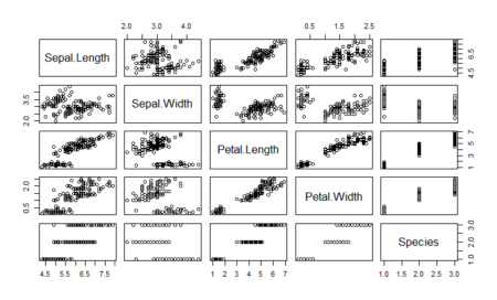
As we can see, one of the classes is completely separate while the other two are somewhat overlapping. However, LDA is still able to distinguish between the two. A better version of using lda is lda() with CV. This can be done by passing the CV=TRUE in the lda function.
#LDA with CV
lda_cv_iris=lda(Species~.,data=dataset,CV=TRUE)

#The predictions are already generated in lda_cv_iris
table(lda_cv_iris$class, dataset$Species)
I didn’t generate the summary for the model as it will also produce all the predictions. As we already know from the summary of lda_iris, the function first calculates the prior probabilities of the classes in the dataset unless provided specifically. The iris dataset had 50 data points for each class hence the prior probabilities are calculated to be 0.33 each. It then makes the necessary calculations which involves means of each class and overall variance and gets the linear discriminant. The function also scales the value of the linear discriminants so that the mean is zero and variance is one. The final value, proportion of trace that we get is the percentage separation that each of the discriminant achieves. Thus, the first linear discriminant is enough and achieves about 99% of the separation.
As a final step, we will plot the linear discriminants and visually see the difference in distinguishing ability. The ldahist() function helps make the separator plot. For the data into the ldahist() function, we can use the x[,1] for the first linear discriminant and x[,2] for the second linear discriminant and so on
#Plot the predictions - first linear discriminant
ldahist(data = Predictions$x[,1], g=Species)
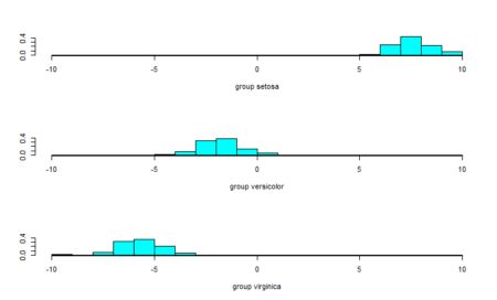
The data points are almost completely separated by the first linear discriminant and that is why we see the three classes in different ranges of values. To further our understanding, we also see the second linear discriminant.
#Plot the predictions - second linear discriminant
ldahist(data = Predictions$x[,2], g=Species)
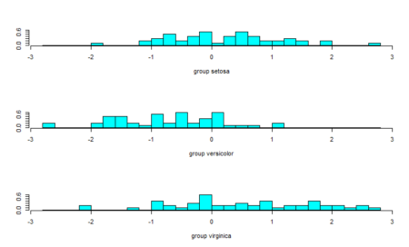
From the plot of the second linear discriminant, we see that we can hardly differentiate between the three groups hence the proportion of trace values.
Everything is not linear – quadratic discriminant analysis
MASS package also contains the qda() function which stands for quadratic discriminant analysis. The idea is simple – if the data can be discriminated using a quadratic function, we can use qda() instead of lda(). The rest of the nuances are the same for qda() as were in lda()
#QDA
qda_iris=qda(Species~.,data=dataset)
qda_iris


Call:
qda(Species ~ ., data = dataset)

Prior probabilities of groups:
            setosa      versicolor      virginica
        0.3333333   0.3333333   0.3333333

Group means:
                Sepal.Length        Sepal.Width         Petal.Length        Petal.Width
setosa              5.006               3.428               1.462               0.246
versicolor          5.936               2.770               4.260               1.326
virginica           6.588               2.974               5.552               2.026

#Check the accuracy of our analysis of qda
Predictions_qda=predict(qda_iris,dataset)
table(Predictions_qda$class, dataset$Species)
                setosa      versicolor  virginica
  setosa            50              0           0
  versicolor        0           48          1
  virginica         0           2           49
Since the data has a linear relation, the qda function also applies the same statistics and returns similar results.
Conclusion: Evaluating LDA and QDA
Even though LDA is a tough problem to understand, its implementation in R is simple. As a final step, we will look into another package- the klaR package which helps to create an exploratory graph for LDA or QDA.
The package contains the partimat() function which takes a similar input as the lda() function but returns a plot instead of the model. The function stands for partition matrix and plots the ability of the features to partition the target class taking combinations of two at a time.
#Using the klarR package
# install.packages("klaR")
library(klaR)
partimat(Species~.,data=dataset,method="lda")
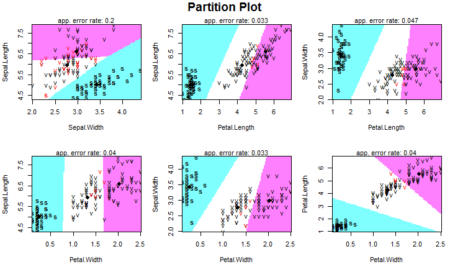
Our data has four features so we have 4C2 =6 combinations to classify our data. The plot show how different classes are defined based on the two features on x-axis and y-axis. As a summary, it is important to know that one should look at the data first to know whether the data seems to be linearly separable (or quadratically separable in case of qda) before selecting the technique. Since LDA makes some assumptions about the data, we also need to preprocess the data and perform univariate analysis to see if the normality assumption holds for each class of the data. In the absence of normality, that is, in case there is a violation of the normality condition, one can still proceed with LDA or QDA but the results will not be appropriate and will lack in accuracy. We also need to analyze whether the features are related to each other and some of them need to be omitted from our analysis. The rest is up to the lda() function to calculate and make predictions on. Here is the entire code used in this article:
#Load the library containing lda() function
library(MASS)
#Store the dataset
dataset=iris

#Help Documentation
?lda

#Perform LDA over the data
lda_iris=lda(Species~.,data=dataset)
#Prior Probabilities and coefficients of Linear discriminants
lda_iris

#Check the accuracy of our analysis
Predictions=predict(lda_iris,dataset)
table(Predictions$class, dataset$Species)

#Check how easily we can linearly separate the iris dataset
pairs(dataset)

#LDA with CV
lda_cv_iris=lda(Species~.,data=dataset,CV=TRUE)

#The predictions are already generated in lda_cv_iris
table(lda_cv_iris$class, dataset$Species)

#Plot the predictions - first linear discriminant
ldahist(data = Predictions$x[,1], g=Species)

#Plot the predictions - second linear discriminant
ldahist(data = Predictions$x[,2], g=Species)

#QDA
qda_iris=qda(Species~.,data=dataset)
qda_iris

#Check the accuracy of our analysis of qda
Predictions_qda=predict(qda_iris,dataset)
table(Predictions_qda$class, dataset$Species)

#Using the klarR packagew
# install.packages("klaR")
library(klaR)
partimat(Species~.,data=dataset,method="lda")
Author Bio:
This article was contributed by Perceptive Analytics. Madhur Modi, Chaitanya Sagar, Jyothirmayee Thondamallu and Saneesh Veetil contributed to this article.
Perceptive Analytics provides data analytics, data visualization, business intelligence and reporting services to e-commerce, retail, healthcare and pharmaceutical industries. Our client roster includes Fortune 500 and NYSE listed companies in the USA and India.