DataCamp is now offering a discount on unlimited access to their course curriculum. Access over 170+ course in R, Python, SQL and more taught by experts and thought-leaders in data science such as Mine Cetinkaya-Rundel (R-Studio), Hadley Wickham (R-Studio), Max Kuhn (caret) and more. Check out this link to get the discount!
Below are some of the tracks available. You can choose a career track which is a deep dive into a subject that covers all the skills needed. Or a skill track which focuses on a specific subject.
Tidyverse Fundamentals (Skill Track)
Experience the whole data science pipeline from importing and tidying data to wrangling and visualizing data to modeling and communicating with data. Gain exposure to each component of this pipeline from a variety of different perspectives in this tidyverse R track.
Finance Basics with R (Skill Track)
If you are just starting to learn about finance and are new to R, this is the right track to kick things off! In this track, you will learn the basics of R and apply your new knowledge directly to finance examples, start manipulating your first (financial) time series, and learn how to pull financial data from local files as well as from internet sources.
Data Scientist with R (Career Track)
A Data Scientist combines statistical and machine learning techniques with R programming to analyze and interpret complex data. This career track gives you exposure to the full data science toolbox.
Quantitative Analyst with R (Career Track)
In finance, quantitative analysts ensure portfolios are risk balanced, help find new trading opportunities, and evaluate asset prices using mathematical models. Interested? This track is for you.
About DataCamp:
DataCamp is an online learning platform that uses high-quality video and interactive in-browser coding challenges to teach you data science using R, Python, SQL and more. All courses can be taken at your own pace. To date, over 2.5+ million data science enthusiasts have already taken one or more courses at DataCamp.
[soundcloud url=”https://api.soundcloud.com/tracks/385794143″ params=”color=#ff5500&auto_play=false&hide_related=false&show_comments=true&show_user=true&show_reposts=false&show_teaser=true&visual=true” width=”100%” height=”300″ iframe=”true” /]
We are super pumped to be launching a weekly data science podcast called DataFramed, in which Hugo Bowne-Anderson (me), a data scientist and educator at DataCamp, speaks with industry experts about what data science is, what it's capable of, what it looks like in practice and the direction it is heading over the next decade and into the future.
You can check out the podcast here and make sure to subscribe, rate and review!
For a sneak peak, check out the trailer above!
Instead of answering "what is data science?" merely through the lens of related technologies, tools and skill-sets, a methodology commonly invoked to discover what data science is, we have decided to answer this question by delving into what modern data science looks like in practice via in-depth conversations with practitioners. These are the types of conversations we all have over dinner, around the water cooler and at conferences and I am happy to be formalizing them and bringing them to you in podcast form.
We're launching with a bang!
We’ve already released 7 episodes, which were honestly so much fun to record. In these episodes, I speak with:
Hilary Mason (VP of Research at Cloudera Fast Forward Labs and Data Scientist in Residence at Accel Partners),
Chris Volinksy (Assistant Vice President for Big Data Research at AT&T Labs and a member of the 7-person, 4-country team that won the $1M Netflix Prize),
Ben Skrainka (data scientist at Convoy, a company dedicated to revolutionizing the North American trucking industry with data science),
Maelle Salmon (Statistician/data scientist in Public Health, Epidemiology, #rstats) and
Dave Robinson (DataCamp, previously StackOverflow).
Robert Chang (Airbnb).
These interviews will be interspersed with brief segments on "Tales from the Open Source", "Statistical Pitfalls", "Data Science blog post of the week" and "Stack Overflow diaries", to name a few. The mission of these segments is to explain and discuss in brief topics essential to any working data scientist's toolbox.
Future episodes will include interviews with Mike Tamir (Head of Data Science Uber ATG), Mara Averick (Tidyverse Dev Advocate, RStudio), Emily Robinson (Etsy) and Drew Conway (Alluvium).
If you have any suggestions or would like to come on the show, do reach out to me on twitter @hugobowne.
Dates and times are abundant in data and essential for answering questions that start with when, how long, or how often. However, they can be tricky, as they come in a variety of formats and can behave in unintuitive ways. This course teaches you the essentials of parsing, manipulating, and computing with dates and times in R. By the end, you'll have mastered the lubridate package, a member of the tidyverse, specifically designed to handle dates and times. You'll also have applied your new skills to explore how often R versions are released, when the weather is good in Auckland (the birthplace of R), and how long monarchs ruled in Britain.
Working with Dates and Times in R features interactive exercises that combine high-quality video, in-browser coding, and gamification for an engaging learning experience that will make you an expert in dates and times in R!
What you'll learn
1. Dates and Times in R
Dates and times come in a huge assortment of formats, so your first hurdle is often to parse the format you have into an R datetime. This chapter teaches you to import dates and times with the lubridate package. You'll also learn how to extract parts of a datetime. You'll practice by exploring the weather in R's birthplace, Auckland NZ.
2. Parsing and Manipulating Dates and Times with lubridate
Dates and times come in a huge assortment of formats, so your first hurdle is often to parse the format you have into an R datetime. This chapter teaches you to import dates and times with the lubridate package. You'll also learn how to extract parts of a datetime. You'll practice by exploring the weather in R's birthplace, Auckland NZ.
3. Arithmetic with Dates and Times
Getting datetimes into R is just the first step. Now that you know how to parse datetimes, you need to learn how to do calculations with them. In this chapter, you'll learn the different ways of representing spans of time with lubridate and how to leverage them to do arithmetic on datetimes. By the end of the chapter, you'll have calculated how long it's been since the first man stepped on the moon, generated sequences of dates to help schedule reminders, calculated when an eclipse occurs, and explored the reigns of monarch's of England (and which ones might have seen Halley's comet!).
4. Problems in practice
You now know most of what you need to tackle data that includes dates and times, but there are a few other problems you might encounter in practice. In this final chapter you'll learn a little more about these problems by returning to some of the earlier data examples and learning how to handle time zones, deal with times when you don't care about dates, parse dates quickly, and output dates and times.
You might have already seen or used the pipe operator when you're working with packages such as dplyr, magrittr,… But do you know where pipes and the famous %>% operator come from, what they exactly are, or how, when and why you should use them? Can you also come up with some alternatives?
This tutorial will give you an introduction to pipes in R and will cover the following topics:
Are you interested in learning more about manipulating data in R with dplyr? Take a look at DataCamp's Data Manipulation in R with dplyr course.
Pipe Operator in R: Introduction
To understand what the pipe operator in R is and what you can do with it, it's necessary to consider the full picture, to learn the history behind it. Questions such as "where does this weird combination of symbols come from and why was it made like this?" might be on top of your mind. You'll discover the answers to these and more questions in this section.
Now, you can look at the history from three perspectives: from a mathematical point of view, from a holistic point of view of programming languages, and from the point of view of the R language itself. You'll cover all three in what follows!
History of the Pipe Operator in R
Mathematical History
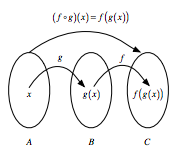
If you have two functions, let's say $f : B → C$ and $g : A → B$, you can chain these functions together by taking the output of one function and inserting it into the next. In short, "chaining" means that you pass an intermediate result onto the next function, but you'll see more about that later.
For example, you can say, $f(g(x))$: $g(x)$ serves as an input for $f()$, while $x$, of course, serves as input to $g()$.
If you would want to note this down, you will use the notation $f ◦ g$, which reads as "f follows g". Alternatively, you can visually represent this as:
As mentioned in the introduction to this section, this operator is not new in programming: in the Shell or Terminal, you can pass command from one to the next with the pipeline character |. Similarly, F# has a forward pipe operator, which will prove to be important later on! Lastly, it's also good to know that Haskell contains many piping operations that are derived from the Shell or Terminal.
Pipes in R
Now that you have seen some history of the pipe operator in other programming languages, it's time to focus on R. The history of this operator in R starts, according to this fantastic blog post written by Adolfo Álvarez, on January 17th, 2012, when an anonymous user asked the following question in this Stack Overflow post:
How can you implement F#'s forward pipe operator in R? The operator makes it possible to easily chain a sequence of calculations. For example, when you have an input data and want to call functions foo and bar in sequence, you can write data |> foo |> bar?
The answer came from Ben Bolker, professor at McMaster University, who replied:
I don't know how well it would hold up to any real use, but this seems (?) to do what you want, at least for single-argument functions …
"%>%" <- function(x,f) do.call(f,list(x))
pi %>% sin
[1] 1.224606e-16
pi %>% sin %>% cos
[1] 1
cos(sin(pi))
[1] 1
About nine months later, Hadley Wickham started the dplyr package on GitHub. You might now know Hadley, Chief Scientist at RStudio, as the author of many popular R packages (such as this last package!) and as the instructor for DataCamp's Writing Functions in R course.
Be however it may, it wasn't until 2013 that the first pipe %.% appears in this package. As Adolfo Álvarez rightfully mentions in his blog post, the function was denominated chain(), which had the purpose to simplify the notation for the application of several functions to a single data frame in R.
The %.% pipe would not be around for long, as Stefan Bache proposed an alternative on the 29th of December 2013, that included the operator as you might now know it:
Bache continued to work with this pipe operation and at the end of 2013, the magrittr package came to being. In the meantime, Hadley Wickham continued to work on dplyr and in April 2014, the %.% operator got replaced with the one that you now know, %>%.
Later that year, Kun Ren published the pipeR package on GitHub, which incorporated a different pipe operator, %>>%, which was designed to add more flexibility to the piping process. However, it's safe to say that the %>% is now established in the R language, especially with the recent popularity of the Tidyverse.
What Is It?
Knowing the history is one thing, but that still doesn't give you an idea of what F#'s forward pipe operator is nor what it actually does in R.
In F#, the pipe-forward operator |> is syntactic sugar for chained method calls. Or, stated more simply, it lets you pass an intermediate result onto the next function.
Remember that "chaining" means that you invoke multiple method calls. As each method returns an object, you can actually allow the calls to be chained together in a single statement, without needing variables to store the intermediate results.
In R, the pipe operator is, as you have already seen, %>%. If you're not familiar with F#, you can think of this operator as being similar to the + in a ggplot2 statement. Its function is very similar to that one that you have seen of the F# operator: it takes the output of one statement and makes it the input of the next statement. When describing it, you can think of it as a "THEN".
Take, for example, following code chunk and read it aloud:
You're right, the code chunk above will translate to something like "you take the Iris data, then you subset the data and then you aggregate the data".
This is one of the most powerful things about the Tidyverse. In fact, having a standardized chain of processing actions is called "a pipeline". Making pipelines for a data format is great, because you can apply that pipeline to incoming data that has the same formatting and have it output in a ggplot2 friendly format, for example.
Why Use It?
R is a functional language, which means that your code often contains a lot of parenthesis, ( and ). When you have complex code, this often will mean that you will have to nest those parentheses together. This makes your R code hard to read and understand. Here's where %>% comes in to the rescue!
Take a look at the following example, which is a typical example of nested code:
class="lang-R"># Initialize `x`
x <- c(0.109, 0.359, 0.63, 0.996, 0.515, 0.142, 0.017, 0.829, 0.907)

# Compute the logarithm of `x`, return suitably lagged and iterated differences,
# compute the exponential function and round the result
round(exp(diff(log(x))), 1)
3.3
1.8
1.6
0.5
0.3
0.1
48.8
1.1
With the help of %<%, you can rewrite the above code as follows:
class="lang-R"># Import `magrittr`
library(magrittr)

# Perform the same computations on `x` as above
x %>% log() %>%
    diff() %>%
    exp() %>%
    round(1)
Does this seem difficult to you? No worries! You'll learn more on how to go about this later on in this tutorial.
Note that you need to import the magrittr library to get the above code to work. That's because the pipe operator is, as you read above, part of the magrittr library and is, since 2014, also a part of dplyr. If you forget to import the library, you'll get an error like Error in eval(expr, envir, enclos): could not find function "%>%".
Also note that it isn't a formal requirement to add the parentheses after log, diff and exp, but that, within the R community, some will use it to increase the readability of the code.
In short, here are four reasons why you should be using pipes in R:
You'll structure the sequence of your data operations from left to right, as apposed to from inside and out;
You'll avoid nested function calls;
You'll minimize the need for local variables and function definitions; And
You'll make it easy to add steps anywhere in the sequence of operations.
These reasons are taken from the magrittr documentation itself. Implicitly, you see the arguments of readability and flexibility returning.
Additional Pipes
Even though %>% is the (main) pipe operator of the magrittr package, there are a couple of other operators that you should know and that are part of the same package:
The compound assignment operator %<>%;
class="lang-R"># Initialize `x`
x <- rnorm(100)

# Update value of `x` and assign it to `x`
x %<>% abs %>% sort
Of course, these three operators work slightly differently than the main %>% operator. You'll see more about their functionalities and their usage later on in this tutorial!
Note that, even though you'll most often see the magrittr pipes, you might also encounter other pipes as you go along! Some examples are wrapr's dot arrow pipe %.>% or to dot pipe %>.%, or the Bizarro pipe ->.;.
How to Use Pipes in R
Now that you know how the %>% operator originated, what it actually is and why you should use it, it's time for you to discover how you can actually use it to your advantage. You will see that there are quite some ways in which you can use it!
Basic Piping
Before you go into the more advanced usages of the operator, it's good to first take a look at the most basic examples that use the operator. In essence, you'll see that there are 3 rules that you can follow when you're first starting out:
f(x) can be rewritten as x %>% f
In short, this means that functions that take one argument, function(argument), can be rewritten as follows: argument %>% function(). Take a look at the following, more practical example to understand how these two are equivalent:
class="lang-R"># Compute the logarithm of `x`
log(x)

# Compute the logarithm of `x`
x %>% log()
f(x, y) can be rewritten as x %>% f(y)
Of course, there are a lot of functions that don't just take one argument, but multiple. This is the case here: you see that the function takes two arguments, x and y. Similar to what you have seen in the first example, you can rewrite the function by following the structure argument1 %>% function(argument2), where argument1 is the magrittr placeholder and argument2 the function call.
This all seems quite theoretical. Let's take a look at a more practical example:
class="lang-R"># Round pi
round(pi, 6)

# Round pi
pi %>% round(6)
x %>% f %>% g %>% h can be rewritten as h(g(f(x)))
This might seem complex, but it isn't quite like that when you look at a real-life R example:
class="lang-R"># Import `babynames` data
library(babynames)
# Import `dplyr` library
library(dplyr)

# Load the data
data(babynames)

# Count how many young boys with the name "Taylor" are born
sum(select(filter(babynames,sex=="M",name=="Taylor"),n))

# Do the same but now with `%>%`
babynames%>%filter(sex=="M",name=="Taylor")%>%
            select(n)%>%
            sum
Note how you work from the inside out when you rewrite the nested code: you first put in the babynames, then you use %>% to first filter() the data. After that, you'll select n and lastly, you'll sum() everything.
Remember also that you already saw another example of such a nested code that was converted to more readable code in the beginning of this tutorial, where you used the log(), diff(), exp() and round() functions to perform calculations on x.
Functions that Use the Current Environment
Unfortunately, there are some exceptions to the more general rules that were outlined in the previous section. Let's take a look at some of them here.
Consider this example, where you use the assign() function to assign the value 10 to the variable x.
class="lang-R"># Assign `10` to `x`
assign("x", 10)

# Assign `100` to `x`
"x" %>% assign(100)

# Return `x`
x
10
You see that the second call with the assign() function, in combination with the pipe, doesn't work properly. The value of x is not updated.
Why is this?
That's because the function assigns the new value 100 to a temporary environment used by %>%. So, if you want to use assign() with the pipe, you must be explicit about the environment:
class="lang-R"># Define your environment
env <- environment()

# Add the environment to `assign()`
"x" %>% assign(100, envir = env)

# Return `x`
x
100
Functions with Lazy Evalution
Arguments within functions are only computed when the function uses them in R. This means that no arguments are computed before you call your function! That means also that the pipe computes each element of the function in turn.
One place that this is a problem is tryCatch(), which lets you capture and handle errors, like in this example:
You'll see that the nested way of writing down this line of code works perfectly, while the piped alternative returns an error. Other functions with the same behavior are try(), suppressMessages(), and suppressWarnings() in base R.
Argument Placeholder
There are also instances where you can use the pipe operator as an argument placeholder. Take a look at the following examples:
f(x, y) can be rewritten as y %>% f(x, .)
In some cases, you won't want the value or the magrittr placeholder to the function call at the first position, which has been the case in every example that you have seen up until now. Reconsider this line of code:
<pi %>% round(6)
If you would rewrite this line of code, pi would be the first argument in your round() function. But what if you would want to replace the second, third, … argument and use that one as the magrittr placeholder to your function call?
Take a look at this example, where the value is actually at the third position in the function call:
class="lang-R">"Ceci n'est pas une pipe" %>% gsub("une", "un", .)
'Ceci n\'est pas un pipe'
f(y, z = x) can be rewritten as x %>% f(y, z = .)
Likewise, you might want to make the value of a specific argument within your function call the magrittr placeholder. Consider the following line of code:
class="lang-R">6 %>% round(pi, digits=.)
Re-using the Placeholder for Attributes
It is straight-forward to use the placeholder several times in a right-hand side expression. However, when the placeholder only appears in a nested expressions magrittr will still apply the first-argument rule. The reason is that in most cases this results more clean code.
Here are some general "rules" that you can take into account when you're working with argument placeholders in nested function calls:
f(x, y = nrow(x), z = ncol(x)) can be rewritten as x %>% f(y = nrow(.), z = ncol(.))
class="lang-R"># Initialize a matrix `ma`
ma <- matrix(1:12, 3, 4)

# Return the maximum of the values inputted
max(ma, nrow(ma), ncol(ma))

# Return the maximum of the values inputted
ma %>% max(nrow(ma), ncol(ma))
12
12
The behavior can be overruled by enclosing the right-hand side in braces:
f(y = nrow(x), z = ncol(x)) can be rewritten as x %>% {f(y = nrow(.), z = ncol(.))}
class="lang-R"># Only return the maximum of the `nrow(ma)` and `ncol(ma)` input values
ma %>% {max(nrow(ma), ncol(ma))}
4
To conclude, also take a look at the following example, where you could possibly want to adjust the workings of the argument placeholder in the nested function call:
class="lang-R"># The function that you want to rewrite
paste(1:5, letters[1:5])

# The nested function call with dot placeholder
1:5 %>%
  paste(., letters[.])
'1 a'
'2 b'
'3 c'
'4 d'
'5 e'
'1 a'
'2 b'
'3 c'
'4 d'
'5 e'
You see that if the placeholder is only used in a nested function call, the magrittr placeholder will also be placed as the first argument! If you want to avoid this from happening, you can use the curly brackets { and }:
class="lang-R"># The nested function call with dot placeholder and curly brackets
1:5 %>% {
  paste(letters[.])
}

# Rewrite the above function call
paste(letters[1:5])
'a'
'b'
'c'
'd'
'e'
'a'
'b'
'c'
'd'
'e'
Building Unary Functions
Unary functions are functions that take one argument. Any pipeline that you might make that consists of a dot ., followed by functions and that is chained together with %>% can be used later if you want to apply it to values. Take a look at the following example of such a pipeline:
class="lang-R">. %>% cos %>% sin
This pipeline would take some input, after which both the cos() and sin() fuctions would be applied to it.
But you're not there yet! If you want this pipeline to do exactly that which you have just read, you need to assign it first to a variable f, for example. After that, you can re-use it later to do the operations that are contained within the pipeline on other values.
class="lang-R"># Unary function
f <- . %>% cos %>% sin

f
structure(function (value)
freduce(value, `_function_list`), class = c("fseq", "function"
))
Remember also that you could put parentheses after the cos() and sin() functions in the line of code if you want to improve readability. Consider the same example with parentheses: . %>% cos() %>% sin().
You see, building functions in magrittr very similar to building functions with base R! If you're not sure how similar they actually are, check out the line above and compare it with the next line of code; Both lines have the same result!
class="lang-R"># is equivalent to
f <- function(.) sin(cos(.))

f
function (.)
sin(cos(.))
Compound Assignment Pipe Operations
There are situations where you want to overwrite the value of the left-hand side, just like in the example right below. Intuitively, you will use the assignment operator <- to do this.
class="lang-R"># Load in the Iris data
iris <- read.csv(url("http://archive.ics.uci.edu/ml/machine-learning-databases/iris/iris.data"), header = FALSE)

# Add column names to the Iris data
names(iris) <- c("Sepal.Length", "Sepal.Width", "Petal.Length", "Petal.Width", "Species")

# Compute the square root of `iris$Sepal.Length` and assign it to the variable
iris$Sepal.Length <-
  iris$Sepal.Length %>%
  sqrt()
However, there is a compound assignment pipe operator, which allows you to use a shorthand notation to assign the result of your pipeline immediately to the left-hand side:
class="lang-R"># Compute the square root of `iris$Sepal.Length` and assign it to the variable
iris$Sepal.Length %<>% sqrt

# Return `Sepal.Length`
iris$Sepal.Length
Note that the compound assignment operator %<>% needs to be the first pipe operator in the chain for this to work. This is completely in line with what you just read about the operator being a shorthand notation for a longer notation with repetition, where you use the regular <- assignment operator.
As a result, this operator will assign a result of a pipeline rather than returning it.
Tee Operations with The Tee Operator
The tee operator works exactly like %>%, but it returns the left-hand side value rather than the potential result of the right-hand side operations.
This means that the tee operator can come in handy in situations where you have included functions that are used for their side effect, such as plotting with plot() or printing to a file.
In other words, functions like plot() typically don't return anything. That means that, after calling plot(), for example, your pipeline would end. However, in the following example, the tee operator %T>% allows you to continue your pipeline even after you have used plot():
Exposing Data Variables with the Exposition Operator
When you're working with R, you'll find that many functions take a data argument. Consider, for example, the lm() function or the with() function. These functions are useful in a pipeline where your data is first processed and then passed into the function.
For functions that don't have a data argument, such as the cor() function, it's still handy if you can expose the variables in the data. That's where the %$% operator comes in. Consider the following example:
With the help of %$% you make sure that Sepal.Length and Sepal.Width are exposed to cor(). Likewise, you see that the data in the data.frame() function is passed to the ts.plot() to plot several time series on a common plot:
In the introduction to this tutorial, you already learned that the development of dplyr and magrittr occurred around the same time, namely, around 2013-2014. And, as you have read, the magrittr package is also part of the Tidyverse.
In this section, you will discover how exciting it can be when you combine both packages in your R code.
For those of you who are new to the dplyr package, you should know that this R package was built around five verbs, namely, "select", "filter", "arrange", "mutate" and "summarize". If you have already manipulated data for some data science project, you will know that these verbs make up the majority of the data manipulation tasks that you generally need to perform on your data.
Take an example of some traditional code that makes use of these dplyr functions:
Both code chunks are fairly long, but you could argue that the second code chunk is more clear if you want to follow along through all of the operations. With the creation of intermediate variables in the first code chunk, you could possibly lose the "flow" of the code. By using %>%, you gain a more clear overview of the operations that are being performed on the data!
In short, dplyr and magrittr are your dreamteam for manipulating data in R!
RStudio Keyboard Shortcuts for Pipes
Adding all these pipes to your R code can be a challenging task! To make your life easier, John Mount, co-founder and Principal Consultant at Win-Vector, LLC and DataCamp instructor, has released a package with some RStudio add-ins that allow you to create keyboard shortcuts for pipes in R. Addins are actually R functions with a bit of special registration metadata. An example of a simple addin can, for example, be a function that inserts a commonly used snippet of text, but can also get very complex!
With these addins, you'll be able to execute R functions interactively from within the RStudio IDE, either by using keyboard shortcuts or by going through the Addins menu.
Note that this package is actually a fork from RStudio's original add-in package, which you can find here. Be careful though, the support for addins is available only within the most recent release of RStudio! If you want to know more on how you can install these RStudio addins, check out this page.
You can download the add-ins and keyboard shortcuts here.
When Not To Use the Pipe Operator in R
In the above, you have seen that pipes are definitely something that you should be using when you're programming with R. More specifically, you have seen this by covering some cases in which pipes prove to be very useful! However, there are some situations, outlined by Hadley Wickham in "R for Data Science", in which you can best avoid them:
Your pipes are longer than (say) ten steps.
In cases like these, it's better to create intermediate objects with meaningful names. It will not only be easier for you to debug your code, but you'll also understand your code better and it'll be easier for others to understand your code.
You have multiple inputs or outputs.
If you aren't transforming one primary object, but two or more objects are combined together, it's better not to use the pipe.
You are starting to think about a directed graph with a complex dependency structure.
Pipes are fundamentally linear and expressing complex relationships with them will only result in complex code that will be hard to read and understand.
You're doing internal package development
Using pipes in internal package development is a no-go, as it makes it harder to debug!
For more reflections on this topic, check out this Stack Overflow discussion. Other situations that appear in that discussion are loops, package dependencies, argument order and readability.
In short, you could summarize it all as follows: keep the two things in mind that make this construct so great, namely, readability and flexibility. As soon as one of these two big advantages is compromised, you might consider some alternatives in favor of the pipes.
Alternatives to Pipes in R
After all that you have read by you might also be interested in some alternatives that exist in the R programming language. Some of the solutions that you have seen in this tutorial were the following:
Create intermediate variables with meaningful names;
Instead of chaining all operations together and outputting one single result, break up the chain and make sure you save intermediate results in separate variables. Be careful with the naming of these variables: the goal should always be to make your code as understandable as possible!
Nest your code so that you read it from the inside out;
One of the possible objections that you could have against pipes is the fact that it goes against the "flow" that you have been accustomed to with base R. The solution is then to stick with nesting your code! But what to do then if you don't like pipes but you also think nesting can be quite confusing? The solution here can be to use tabs to highlight the hierarchy.
… Do you have more suggestions? Make sure to let me know – Drop me a tweet @willems_karlijn
Conclusion
You have covered a lot of ground in this tutorial: you have seen where %>% comes from, what it exactly is, why you should use it and how you should use it. You've seen that the dplyr and magrittr packages work wonderfully together and that there are even more operators out there! Lastly, you have also seen some cases in which you shouldn't use it when you're programming in R and what alternatives you can use in such cases.
If you're interested in learning more about the Tidyverse, consider DataCamp's Introduction to the Tidyverse course.
This is an introduction to the programming language R, focused on a powerful set of tools known as the “tidyverse”. In the course you’ll learn the intertwined processes of data manipulation and visualization through the tools dplyr and ggplot2. You’ll learn to manipulate data by filtering, sorting and summarizing a real dataset of historical country data in order to answer exploratory questions. You’ll then learn to turn this processed data into informative line plots, bar plots, histograms, and more with the ggplot2 package. This gives a taste both of the value of exploratory data analysis and the power of tidyverse tools. This is a suitable introduction for people who have no previous experience in R and are interested in learning to perform data analysis.
Take me to chapter 1!
Introduction to the Tidyverse features interactive exercises that combine high-quality video, in-browser coding, and gamification for an engaging learning experience that will make you a Tidyverse expert!
What you’ll learn
1. Data wrangling
In this chapter, you’ll learn to do three things with a table: filter for particular observations, arrange the observations in a desired order, and mutate to add or change a column. You’ll see how each of these steps lets you answer questions about your data.
2. Data visualization
You’ve already been able to answer some questions about the data through dplyr, but you’ve engaged with them just as a table (such as one showing the life expectancy in the US each year). Often a better way to understand and present such data is as a graph. Here you’ll learn the essential skill of data visualization, using the ggplot2 package. Visualization and manipulation are often intertwined, so you’ll see how the dplyr and ggplot2 packages work closely together to create informative graphs.
3. Grouping and summarizing
So far you’ve been answering questions about individual country-year pairs, but we may be interested in aggregations of the data, such as the average life expectancy of all countries within each year. Here you’ll learn to use the group by and summarize verbs, which collapse large datasets into manageable summaries.
4. Types of visualizations
You’ve learned to create scatter plots with ggplot2. In this chapter you’ll learn to create line plots, bar plots, histograms, and boxplots. You’ll see how each plot needs different kinds of data manipulation to prepare for it, and understand the different roles of each of these plot types in data analysis.
Hi there! We just launched Working with Web Data in R by Oliver Keyes and Charlotte Wickham, our latest R course!
Most of the useful data in the world, from economic data to news content to geographic information, lives somewhere on the internet – and this course will teach you how to access it. You’ll explore how to work with APIs (computer-readable interfaces to websites), access data from Wikipedia and other sources, and build your own simple API client. For those occasions where APIs are not available, you’ll find out how to use R to scrape information out of web pages. In the process, you’ll learn how to get data out of even the most stubborn website, and how to turn it into a format ready for further analysis. The packages you’ll use and learn your way around are rvest, httr, xml2 and jsonlite, along with particular API client packages like WikipediR and pageviews.
Working with Web Data in R features interactive exercises that combine high-quality video, in-browser coding, and gamification for an engaging learning experience that will make you an expert in getting information from the Internet!
What you’ll learn
1. Downloading Files and Using API Clients
Sometimes getting data off the internet is very, very simple – it’s stored in a format that R can handle and just lives on a server somewhere, or it’s in a more complex format and perhaps part of an API but there’s an R package designed to make using it a piece of cake. This chapter will explore how to download and read in static files, and how to use APIs when pre-existing clients are available.
2. Using httr to interact with APIs directly
If an API client doesn’t exist, it’s up to you to communicate directly with the API. But don’t worry, the package httr makes this really straightforward. In this chapter, you’ll learn how to make web requests from R, how to examine the responses you get back and some best practices for doing this in a responsible way.
3. Handling JSON and XML
Sometimes data is a TSV or nice plaintext output. Sometimes it’s XML and/or JSON. This chapter walks you through what JSON and XML are, how to convert them into R-like objects, and how to extract data from them. You’ll practice by examining the revision history for a Wikipedia article retrieved from the Wikipedia API using httr, xml2 and jsonlite.
4. Web scraping with XPATHs
Now that we’ve covered the low-hanging fruit (“it has an API, and a client”, “it has an API”) it’s time to talk about what to do when a website doesn’t have any access mechanisms at all – when you have to rely on web scraping. This chapter will introduce you to the rvest web-scraping package, and build on your previous knowledge of XML manipulation and XPATHs.
5. ECSS Web Scraping and Final Case Study
CSS path-based web scraping is a far-more-pleasant alternative to using XPATHs. You’ll start this chapter by learning about CSS, and how to leverage it for web scraping. Then, you’ll work through a final case study that combines everything you’ve learnt so far to write a function that queries an API, parses the response and returns data in a nice form.