Using Shiny Dashboards for Financial Analysis

For some time now, I have been trading traditional assets—mostly U.S. equities. About a year ago, I jumped into the cryptocurrency markets to try my hand there as well. In my time in investor Telegram chats and subreddits, I often saw people arguing over which investments had performed better over time, but the reality was that most such statements were anecdotal, and thus unfalsifiable.

Given the paucity of cryptocurrency data available in an easily accessible format, it was quite difficult to say for certain that a particular investment was a good one relative to some alternative, unless you were very familiar with a handful of APIs. Even then, assuming you knew how to get daily OHLC data for a crypto-asset like Bitcoin, in order to compare it to some other asset—say Amazon stock—you would have to eyeball trends from a website like Yahoo finance or scrape that data separately and build your own visualizations and metrics. In short, historical asset performance comparisons in the crypto space were difficult to conduct for all but the most technically savvy individuals, so I set out to build a tool that would remedy this, and the Financial Asset Comparison Tool was born.

In this post, I aim to describe a few key components of the dashboard, and also call out lessons learned from the process of iterating on the tool along the way. Prior to proceeding, I highly recommend that you read the app’s README and take a look at the UI and code base itself, as this will provide the context necessary to understanding the rest of the commentary below.


I’ll start by delving into a few principles that I find to be to key when designing analytic dashboards, drawing on the asset comparison dashboard as my exemplar, and will end with some discussion of the relative utility of a few packages integral to the app. Overall, my goal is not to focus on the tool that I built alone, but to highlight a few main best practices when it comes to building dashboards for any analysis.

Build the app around the story, not the other way around.


Before ever writing a single line of code for an analytic app, I find that it is absolutely imperative to have a clear vision of the story that the tool must tell. I do not mean by this that you should already have conclusions about your data that you will then force the app into telling, but rather, that you must know how you want your user to interact with the app in order glean useful information.

In the case of my asset comparison tool, I wanted to serve multiple audiences—everyone from a casual trader who just wanted to see which investment produced the greatest net profit over a period of time, to a more experience trader, who had more nuanced questions about risk-adjusted return on investment given varying discount rates. The trick is thus building the app in such a way that serves all possible audiences without hindering any one type of user in particular.

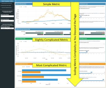
The way I designed my app to meet this need was to build the UI such that as you descend the various sections vertically, the metrics displayed scale in complexity. My reasoning for this becomes apparent when you consider the two extremes in terms of users—the most basic vs. the most advanced trader.

The most basic user will care only about the assets of interest, the time period they want to examine, and how their initial investment performed over time. As such, they will start with the sidebar, input their assets and time frame of choice, and then use the top right-most input box to modulate their initial investment amount (although some may choose to stick with the default value here). They will then see the first chart change to reflect their choices, and they will see, both visually, and via the summary table below, which asset performed better.

The experienced trader, on the other hand, will start off exactly as the novice did, by choosing assets of interest, a time frame of reference, and an initial investment amount. They may then choose to modulate the LOESS parameters as they see fit, descending the page, looking over the simple returns section, perhaps stopping to make changes to the corresponding inputs there, and finally ending at the bottom of the page—at the Sharpe Ratio visualizations. Here they will likely spend more time—playing around with the time period over which to measure returns and changing the risk-free rate to align with their own personal macroeconomic assumptions.

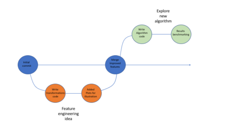
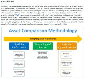
The point of these two examples is to illustrate that the app by dint of its structure alone guides the user through the analytic story in a waterfall-like manner—building from simple portfolio performance, to relative performance, to the most complicated metrics for risk-adjusted returns. This keeps the novice trader from being overwhelmed or confused, and also allows the most experienced user to follow the same line of thought that they would anyway when comparing assets, while following a logical progression of complexity, as shown via the screenshot below.


Once you think you have a structure that guides all users through the story you want them to experience, test it by asking yourself if the app flows in such a way that you could pose and answer a logical series of questions as you navigate the app without any gaps in cohesion. In the case of this app, the questions that the UI answers as you descend are as follows:


  • How do these assets compare in terms of absolute profit?
  • How do these assets compare in terms of simple return on investment?
  • How do these assets compare in terms of variance-adjusted and/or risk-adjusted return on investment?


Thus, when you string these questions together, you can make statements of the type: “Asset X seemed to outperform Asset Y in terms of absolute profit, and this trend held true as well when it comes to simple return on investment, over varying time frames. That said, when you take into account the variance inherent to Asset X, it seems that Asset Y may have been the best choice, as the excess downside risk associated with Asset X outweighs its excess net profitability.


Too many cooks in the kitchen—the case for a functional approach to app-building.


While the design of the UI of any analytic app is of great importance, it’s important to not forget that the code base itself should also be well-designed; a fully-functional app from the user’s perspective can still be a terrible app to work with if the code is a jumbled, incomprehensible mess. A poorly designed code base makes QC a tiresome, aggravating process, and knowledge sharing all but impossible.

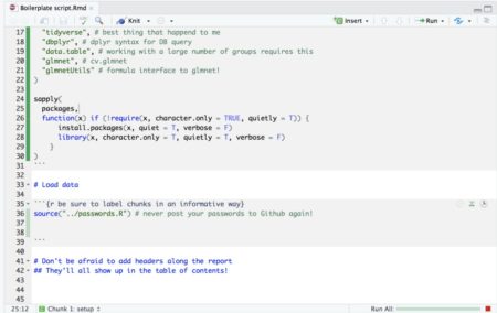
For this reason, I find that sourcing a separate R script file containing all analytic functions necessitated by the app is the best way to go, as done below (you can see Functions.R at my repo here).


# source the Functions.R file, where all analytic functions for the app are stored
source("Functions.R")


Not only does this allow for a more comprehensible and less-cluttered App.R, but it also drastically improves testability and reusability of the code. Consider the example function below, used to create the portfolio performance chart in the app (first box displayed in the UI, center middle).

build_portfolio_perf_chart <- function(data, port_loess_param = 0.33){
  
  port_tbl <- data[,c(1,4:5)]
  
  # grabbing the 2 asset names
  asset_name1 <- sub('_.*', '', names(port_tbl)[2])
  asset_name2 <- sub('_.*', '', names(port_tbl)[3])
  
  # transforms dates into correct type so smoothing can be done
  port_tbl[,1] <- as.Date(port_tbl[,1])
  date_in_numeric_form <- as.numeric((port_tbl[,1]))
  # assigning loess smoothing parameter
  loess_span_parameter <- port_loess_param
  
  # now building the plotly itself
  port_perf_plot <- plot_ly(data = port_tbl, x = ~port_tbl[,1]) %>%
    # asset 1 data plotted
    add_markers(y =~port_tbl[,2],
                marker = list(color = '#FC9C01'),
                name = asset_name1,
                showlegend = FALSE) %>%
    add_lines(y = ~fitted(loess(port_tbl[,2] ~ date_in_numeric_form, span = loess_span_parameter)),
              line = list(color = '#FC9C01'),
              name = asset_name1,
              showlegend = TRUE) %>%
    # asset 2 data plotted
    add_markers(y =~port_tbl[,3],
                marker = list(color = '#3498DB'),
                name = asset_name2,
                showlegend = FALSE) %>%
    add_lines(y = ~fitted(loess(port_tbl[,3] ~ date_in_numeric_form, span = loess_span_parameter)),
              line = list(color = '#3498DB'),
              name = asset_name2,
              showlegend = TRUE) %>%
    layout(
      title = FALSE,
      xaxis = list(type = "date",
                   title = "Date"),
      yaxis = list(title = "Portfolio Value ($)"),
      legend = list(orientation = 'h',
                    x = 0,
                    y = 1.15)) %>%
    add_annotations(
      x= 1,
      y= 1.133,
      xref = "paper",
      yref = "paper",
      text = "",
      showarrow = F
    )
  
  return(port_perf_plot)
  
}


Writing this function in the sourced Functions.R file instead of directly within the App.R allows for the developer to first test the function itself with fake data—i.e. data not gleaned from the reactive inputs. Once it has been tested in this way, it can be integrated in the app.R on the server side as shown below, with very little code.

  output$portfolio_perf_chart <- 
    debounce(
      renderPlotly({
        data <- react_base_data()
        build_portfolio_perf_chart(data, port_loess_param = input$port_loess_param)
      }), 
      millis = 2000) # sets wait time for debounce


This process allows for better error-identification and troubleshooting. If, for example, you want to change the work accomplished by the analytic function in some way, you can make the changes necessary to the code, and if the app fails to produce the desired outcome, you simply restart the chain: first you test the function in a vacuum outside of the app, and if it runs fine there, then you know that you have a problem with the way the reactive inputs are integrating with the function itself. This is a huge time saver when debugging.

Lastly, this allows for ease of reproducibility and hand-offs. If, say, one of your functions simply takes in a dataset and produces a chart of some sort, then it can be easily copied from the Functions.R and reused elsewhere. I have done this too many times to count, ripping code from project and, with a few alterations, instantly applying it in other contexts. This is easy to do if the functions are written in a manner not dependent on a particular Shiny reactive structure. For all these reasons, it makes sense in most cases to keep the code for the app UI and inputs cleanly separated from the analytic functions via a sourced R script.

Dashboard documentation—both a story and a manual, not one or the other.


When building an app for a customer at work, I never simply write an email with a link in it and write “here you go!” That will result in, at best, a steep learning curve, and at worst, an app used in an unintended way, resulting in user frustration or incorrect results. I always meet with the customer, explain the purpose and functionalities of the tool, walk through the app live, take feedback, and integrate any key takeaways into further iterations.

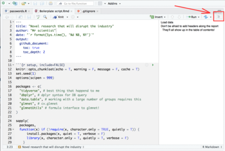
Even if you are just planning on writing some code to put up on GitHub, you should still consider all of these steps when working on the documentation for your app. In most cases, the README is the epicenter of your documentation—the README is your meeting with the customer.  As you saw when reading the 
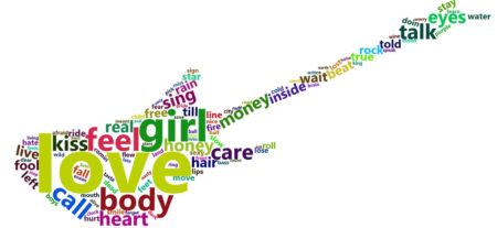
README for the Asset Comparison Tool, I always start my READMEs with a high-level introduction to the purpose of the app—hopefully written or supplemented with visuals (as seen below) that are easy to understand and will capture the attention of browsing passers-by. 


After this introduction, the rest of the potential sections to include can vary greatly from app-to-app. In some cases apps are meant to answer one particular question, and might have a variety of filters or supplemental functionalities—one such example can be found here. As can be seen, in that README, I spend a great deal of time on the methodology after making the overall purpose clear, calling out additional options along the way. In the case of the README for the Asset Comparison Tool, however, the story is a bit different. Given that there are many questions that the app seeks to answer, it makes sense to answer each in turn, writing the README in such a way that its progression mirrors the logical flow of the progression intended for the app’s user.

One should of course not neglect to cover necessary technical information in the README as well. Anything that is not immediately clear from using the app should be clarified in the README—from calculation details to the source of your data, etc. Finally, don’t neglect the iterative component! Mention how you want to interact with prospective users and collaborators in your documentation. For example, I normally call out how I would like people to use the Issues tab on GitHub to propose any changes or additions to the documentation, or the app in general. In short, your documentation must include both the story you want to tell, and a manual for your audience to follow. 

Why Shiny Dashboard?


One of the first things you will notice about the app.R code is that the entire thing is built using Shiny Dashboard as its skeleton. There are a two main reasons for this, which I will touch on in turn.

Shiny Dashboard provides the biggest bang for your buck in terms of how much UI complexity and customizability you get out of just a small amount of code.


I can think of few cases where any analyst or developer would prefer longer, more verbose code to a shorter, succinct solution. That said, Shiny Dashboard’s simplicity when it comes to UI manipulation and customization is not just helpful because it saves you time as a coder, but because it is intuitive from the perspective of your audience.

Most of the folks that use the tools I have built to shed insight into economic questions don’t know how to code in R or Python, but they can, with a little help from extensive commenting and detailed documentation, understand the broad structure of an app coded in Shiny Dashboard format. This is, I believe, largely a function of two features of Shiny Dashboard: the colloquial-English-like syntax of the code for UI elements, and the lack of the necessity for in-line or external CSS.

As you can see from the example below, Shiny Dashboard’s system of “boxes” for UI building is easy to follow. Users can see a box in the app and easily tie that back to a particular box in the UI code.

Here is the box as visible to the user:


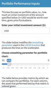
And here is the code that produces the box:

box(
        title = "Portfolio Performance Inputs",
        status= "primary",
        solidHeader = TRUE,
        h5("This box focuses on portfolio value, i.e., how much an initial investment of the amount specified below (in USD) would be worth over time, given price fluctuations."),
        
        textInput(
          inputId = "initial_investment",
          label = "Enter your initial investment amount ($):",
          value = "1000"),
        
        hr(),
        
        h5("The slider below modifies the", a(href = "https://stats.stackexchange.com/questions/2002/how-do-i-decide-what-span-to-use-in-loess-regression-in-r", "smoothing parameter"), "used in the", a(href = "https://en.wikipedia.org/wiki/Local_regression", "LOESS function"), "that produces the lines on the scatterplot."),
        
        sliderInput(
          inputId = "port_loess_param",
          label = "Smoothing parameter for portfolio chart:",
          min = 0.1,
          max = 2,
          value = .33,
          step = 0.01,
          animate = FALSE
        ),
        
        hr(),
        h5("The table below provides metrics by which we can compare the portfolios. For each column, the asset that performed best by that metric is colored green."),
        
        height = 500, 
        width = 4
      )


Secondly, and somewhat related to the first point, with Shiny Dashboard, much of the coloring and overall UI design comes pre-made via dashboard-wide “skins”, and box-specific “statuses.”

This is great if you are okay sacrificing a bit of control for a significant reduction in code complexity. In my experience dealing with non-coding-proficient audiences, I find that in-line CSS or complicated external CSS makes folks far more uncomfortable with the code in general. Anything you can do to reduce this anxiety and make those using your tools feel as though they understand them better is a good thing, and Shiny Dashboard makes that easier.

Shiny Dashboard’s combination of sidebar and boxes makes for easy and efficient data processing when your app has a waterfall-like analytic structure. 


Having written versions of this app both in base Shiny and using Shiny Dashboard, the number one reason I chose Shiny Dashboard was the fact that the analytic questions I sought to solve followed a waterfall-like structure, as explained in the previous section. This works perfectly well with Shiny Dashboard’s combination of sidebar input controls and inputs within UI boxes themselves.  

The inputs of primordial importance to all users are included in the sidebar UI: the two assets to analyze, and the date range over which to compare their performance. These are the only inputs that all users, regardless of experience or intent, must absolutely use, and when they are changed, all views in the dashboard will be affected. All other inputs are stored in the UI Boxes adjacent to the views that they modulate. This makes for a much more intuitive and fluid user experience, as once the initial sidebar inputs have been modulated, the sidebar can be hidden, as all other non-hidden inputs affect only the visualizations to which they are adjacent.

This waterfall-like structure also makes for more efficient reactive processes on the Shiny back-end. The inputs on the sidebar are parameters that, when changed, force the main reactive function that creates that primary dataset to fire, thus recreating the base dataset (as can be seen in the code for that base datasets creation below).

  # utility functions to be used within the server; this enables us to use a textinput for our portfolio values
  exists_as_number <- function(item) {
    !is.null(item) && !is.na(item) && is.numeric(item)
  }
  
  # data-creation reactives (i.e. everything that doesn't directly feed an output)
  
  # first is the main data pull which will fire whenever the primary inputs (asset_1a, asset_2a, initial_investment, or port_dates1a change)
  react_base_data <- reactive({
    if (exists_as_number(as.numeric(input$initial_investment)) == TRUE) {
      # creates the dataset to feed the viz
      return(
        get_pair_data(
          asset_1 = input$asset_1a,
          asset_2 = input$asset_2a, 
          port_start_date = input$port_dates1a[1],
          port_end_date = input$port_dates1a[2],
          initial_investment = (as.numeric(input$initial_investment))
        )
      )
    } else {
      return(
        get_pair_data(
          asset_1 = input$asset_1a,
          asset_2 = input$asset_2a, 
          port_start_date = input$port_dates1a[1],
          port_end_date = input$port_dates1a[2],
          initial_investment = (0)
        )
      )
    }
  })


Each of the visualizations are then produced via their own separate reactive functions, each of which takes as an input the main reactive (as shown below). This makes it so that whenever the sidebar inputs are changed, all reactives fire and all visualizations are updated; however, if all that is changed is a single loess smoothing parameter input, only the reactive used in the creation of that particular parameter-dependent visualization fires, which makes for great computational efficiency.

 # Now the reactives for the actual visualizations
  output$portfolio_perf_chart <- 
    debounce(
      renderPlotly({
        data <- react_base_data()
        build_portfolio_perf_chart(data, port_loess_param = input$port_loess_param)
      }), 
      millis = 2000) # sets wait time for debounce


Why Plotly?


Plotly vs. ggplot is always a fun subject for discussion among folks who build visualizations in R. Sometimes I feel like such discussions just devolve into the same type of argument as R vs. Python for data science (my answer to this question being just pick one and learn it well), but over time I have found that there are actually some circumstances where the plotly vs. ggplot debate can yield cleaner answers.

In particular, I have found in working on this particular type of analytic app that there are two areas where plotly has a bit of an advantage: clickable interactivity, and wide data.

Those familiar with ggplot will know that every good ggplot begins with long data. It is possible, via some functions, to transform wide data into a long format, but that transformation can sometimes be problematic. While there are essentially no circumstances in which it is impossible to transform wide data into long format, there are a handful of cases where it is excessively cumbersome: namely, when dealing with indexed xts objects (as shown below) or time series / OHLC-styled data.


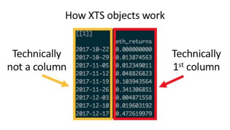
In these cases—either due to the sometimes-awkward way in which you have to handle rowname indexes in xts, or the time and code complexity saved by not having to transform every dataset into long format—plotly offers efficiency gains relative to ggplot.

The aforementioned efficiency gains are a reason to choose plotly in some cases because it makes the life of the coder easier, but there are also reasons why it sometimes make the life of the user easier as well.

If one of the primary utilities of a visualization is to allow the user the ability to seamlessly and intuitively zoom in on, select, or filter the data displayed, particularly in the context of a Shiny App, then plotly should be strongly considered. Sure, ggplotly wrappers can be used to make a ggplot interactive, but with an added layer of abstraction comes an added layer of possible errors. While in most cases a ggplotly wrapper should work seamlessly, I have found that, particularly in cases where auto-sizing and margin size specification is key, ggplotly can require a great deal of added code in order to work correctly in a Shiny context.

In summary, when considering when to start with plotly vs. when to start with ggplot, I find one question to be particularly helpful: what do I value most—visual complexity and/or customization, or interactive versatility and/or preserving wide data?


If I choose the former, then ggplot is what I need; otherwise, I go with plotly. More often than not I find that ggplot emerges victorious, but even if you disagree with me in my decision-making calculus, I think it is helpful to at least think through what your personal calculus is. This will save you time when coding, as instead of playing around with various types of viz, you can simply pose the question(s) behind your calculus and know quickly what solution best fits your problem.

Why Formattable?


The case for formattable is, in my opinion, a much easier case to make than arguing for plotly vs. ggplot. The only question worth asking when deciding on whether or not to use formattable in your app is: do I want my table to tell a quick story via added visual complexity within the same cell that contains my data, or is a reference table all I am looking for? If you chose the former, formattable is probably a good way to go. You’ll notice as well that the case for formattable is very specific–in most cases there is likely a simpler solution via the DT  or kableExtra packages.


The one downside that I have encountered in dealing with formattable code is the amount of code necessary to generate even moderately complicated tables. That said, this problem is easily remedied via a quick function that we can use to kill most of the duplicative coding, as seen in the example below.


First, here is the long form version:


  react_formattable <- reactive({
    return(
      formattable(react_port_summary_table(), 
                  list(
                    "Asset Portfolio Max Worth" = formatter("span",
                                                            style = x ~ style(
                                                              display = "inline-block",
                                                              direction = "rtl",
                                                              "border-radius" = "4px",
                                                              "padding-right" = "2px",
                                                              "background-color" = csscolor("darkslategray"),
                                                              width = percent(proportion(x)),
                                                              color = csscolor(gradient(x, "red", "green"))
                                                            )),
                    "Asset Portfolio Latest Worth" = formatter("span",
                                                               style = x ~ style(
                                                                 display = "inline-block",
                                                                 direction = "rtl",
                                                                 "border-radius" = "4px",
                                                                 "padding-right" = "2px",
                                                                 "background-color" = csscolor("darkslategray"),
                                                                 width = percent(proportion(x)),
                                                                 color = csscolor(gradient(x, "red", "green"))
                                                               )),
                    "Asset Portfolio Absolute Profit" = formatter("span",
                                                                  style = x ~ style(
                                                                    display = "inline-block",
                                                                    direction = "rtl",
                                                                    "border-radius" = "4px",
                                                                    "padding-right" = "2px",
                                                                    "background-color" = csscolor("darkslategray"),
                                                                    width = percent(proportion(x)),
                                                                    color = csscolor(gradient(x, "red", "green"))
                                                                  )),
                    "Asset Portfolio Rate of Return" = formatter("span",
                                                                 style = x ~ style(
                                                                   display = "inline-block",
                                                                   direction = "rtl",
                                                                   "border-radius" = "4px",
                                                                   "padding-right" = "2px",
                                                                   "background-color" = csscolor("darkslategray"),
                                                                   width = percent(proportion(x)),
                                                                   color = csscolor(gradient(x, "red", "green"))
                                                                 ))
                    
                  )
      )
      
    )
  })


This code can easily be shortened via the integration of a custom function, as shown below.


simple_formatter <- function(){
    formatter("span",
              style = x ~ style(
                display = "inline-block",
                direction = "rtl",
                "border-radius" = "4px",
                "padding-right" = "2px",
                "background-color" = csscolor("darkslategray"),
                width = percent(proportion(x)),
                color = csscolor(gradient(x, "red", "green"))
              ))
  }
  
  react_formattable <- reactive({
    return(
      formattable(react_port_summary_table(), 
                  list(
                    "Asset Portfolio Max Worth" = simple_formatter(),
                    "Asset Portfolio Latest Worth" = simple_formatter(),
                    "Asset Portfolio Absolute Profit" = simple_formatter(),
                    "Asset Portfolio Rate of Return" = simple_formatter()
                    )
                  )
      )
    })


As can be seen, formattable allows for a great deal of added complexity in crafting your table—complexity that may not be suited for all apps. That said, if you do want to quickly draw a user’s attention to something in a table, formattable is a great solution, and most of the details of the code can be greatly simplified via a function, as shown.

Conclusions:


That was a lot—I know—but I hope that from this commentary and my exemplar of the Asset Comparison Tool more generally has helped to inform your understanding of how dashboards can serve as a helpful analytic tool. Furthermore, I hope to have prompted some thoughts as to the best practices to be followed when building such a tool. I’ll end with a quick tl;dr:


  • Shave complexity wherever possible, and make code as simple as possible by keeping the code for the app’s UI and inner mechanism (inputs, reactives, etc.) separate from the code for the analytic functions and visualizations.
  • Build with the most extreme cases in mind (think of how your most edge-case user might use the app, and ensure that behavior won’t break the app)
  • Document, document, and then document some more. Make your README both a story and a manual.
  • Give Shiny Dashboard a shot if you want an easy-to-construct UI over which you don’t need complete control when it comes to visual design.
  • Pick your visualization packages based on what you want to prioritize for your user, not the other way around (this applies to ggplot, plotly, formattable, etc.).

Thanks for reading!

Discriminant Analysis: Statistics All The Way

Discriminant analysis is used when the variable to be predicted is categorical in nature. This analysis requires that the way to define data points to the respective categories is known which makes it different from cluster analysis where the classification criteria is not know. It works by calculating a score based on all the predictor variables and based on the values of the score, a corresponding class is selected. Hence, the name discriminant analysis which, in simple terms, discriminates data points and classifies them into classes or categories based on analysis of the predictor variables. This article delves into the linear discriminant analysis function in R and delivers in-depth explanation of the process and concepts. Before we move further, let us look at the assumptions of discriminant analysis which are quite similar to MANOVA.

  • Since we are dealing with multiple features, one of the first assumptions that the technique makes is the assumption of multivariate normality that means the features are normally distributed when separated for each class. This also implies that the technique is susceptible to possible outliers and is also sensitive to the group sizes. If there is an imbalance between the group sizes and one of the groups is too small or too large, the technique suffers when classifying data points into that ‘outlier’ class
  • The second assumption is about homoscedasticity. This states that the variance of the features is same across all the classes of the predictor feature
  • We also assume that the features are sampled randomly
  • The final assumption is about the absence of multicollinearity. If the variables are correlated with each other, the predictive ability will decrease.
Though the discriminant analysis can discriminate features non-linearly as well, linear discriminant analysis is a simpler and more popular methodology. We have normally distributed conditional probability functions for each class. If y is the class to be predicted with two values, 1 and 2 and x is the combined set of all the predictor features, we can assume a threshold value T such that the value which comes as a result of linear combination of features of x belongs to class 1 if it is less than T and belongs to class 2 otherwise. Mathematically,

(x−μ1)TΣ1−1(x−μ1)+ln|Σ1|−(x−μ2)TΣ2−1(x−μ2)−ln|Σ2|T

Where (μ1,Σ1) and(μ2, Σ2) are the respective means and variances of x for class 1 and class 2. We sometimes simplify our calculations by assuming equal variances of the two classes to get a simplified version w.x>c where c is the threshold and w is the weight combined with x.

Let’s understand Fisher’s LDA which is one of the most popular variants of LDA

Fisher’s Linear Discriminant analysis – How and when to use it?

Fisher’s linear discriminant finds out a linear combination of features that can be used to discriminate between the target variable classes. In Fisher’s LDA, we take the separation by the ratio of the variance between the classes to the variance within the classes. To understand it in a different way, it is the interclass variance to intraclass variance ratio
S= 𝛔2between/𝛔2within = (w⋅(μ2−μ1))2/ wT(Σ1+Σ2)w
Fisher’s LDA maximizes this ratio and has a lot of applications. One of the recent applications involve classification of speech and audio. Other past usages include face recognition where Fisher’s LDA is used to create Fisher’s Faces and combined with PCA technique to get eigenfaces. Fisher’s LDA also finds usages in earth science, biomedical science, bankruptcy problems and finance along with in marketing. That’s all on the theoretical aspect of LDA. Let’s understand using an example in R.

LDA Classification example in R

R has a MASS package which has the lda() function. For dataset, we will use the iris dataset and try to classify the classes.
#Load the library containing lda() function
library(MASS)
#Store the dataset
dataset=iris

Before running the lda() function, let’s start with the help documentation of lda()
#Help Documentation
?lda
The description for lda() is minimalistic and simple. We are interested in the details section of the documentation which describes the process which the function uses. As the documentation mentions – the lda() function also tries to detect if the within-class covariance matrix is singular. We can also define a tolerance such that if any variable has within-group variance less than tol^2 it will stop and report the variable as a constant. Another possible adjustment is the prior probabilities. The prior parameter in lda() function is used to specify the prior probabilities. If not specified, the function calculates the prior probabilities to be the same as the distribution of classes in the data. These prior probabilities also affect the rotation of the linear discriminants. Let us proceed with performing linear discriminant analysis over the iris dataset.
#Perform LDA over the data
lda_iris=lda(Species~.,data=dataset)
#Prior Probabilities and coefficients of Linear discriminants
lda_iris

Call:
lda(Species ~ ., data = dataset)

Prior probabilities of groups:
        setosa      versicolor      virginica 
    0.3333333   0.3333333   0.3333333 

Group means:
                Sepal.Length        Sepal.Width         Petal.Length        Petal.Width
setosa              5.006               3.428               1.462               0.246
versicolor          5.936               2.770               4.260               1.326
virginica           6.588               2.974               5.552               2.026

Coefficients of linear discriminants:
                            LD1             LD2
Sepal.Length        0.8293776   0.02410215
Sepal.Width         1.5344731   2.16452123
Petal.Length        -2.2012117  -0.93192121
Petal.Width         -2.8104603      2.83918785

Proportion of trace:
        LD1         LD2 
0.9912  0.0088 


#Check the accuracy of our analysis
Predictions=predict(lda_iris,dataset)
table(Predictions$class, dataset$Species)
                setosa      versicolor  virginica
  setosa            50              0           0
  versicolor        0           48          1
  virginica         0           2           49
With LDA, we are able to classify all but 3 data points correctly in iris dataset. This is probably because the iris data is linearly separable. How do we know whether a data is linearly separable or not? We use the pairs function to see the scatter plots of data and see if they are separable
#Check how easily we can linearly separate the iris dataset
pairs(dataset)

As we can see, one of the classes is completely separate while the other two are somewhat overlapping. However, LDA is still able to distinguish between the two. A better version of using lda is lda() with CV. This can be done by passing the CV=TRUE in the lda function.
#LDA with CV
lda_cv_iris=lda(Species~.,data=dataset,CV=TRUE)

#The predictions are already generated in lda_cv_iris
table(lda_cv_iris$class, dataset$Species)
I didn’t generate the summary for the model as it will also produce all the predictions. As we already know from the summary of lda_iris, the function first calculates the prior probabilities of the classes in the dataset unless provided specifically. The iris dataset had 50 data points for each class hence the prior probabilities are calculated to be 0.33 each. It then makes the necessary calculations which involves means of each class and overall variance and gets the linear discriminant. The function also scales the value of the linear discriminants so that the mean is zero and variance is one. The final value, proportion of trace that we get is the percentage separation that each of the discriminant achieves. Thus, the first linear discriminant is enough and achieves about 99% of the separation. As a final step, we will plot the linear discriminants and visually see the difference in distinguishing ability. The ldahist() function helps make the separator plot. For the data into the ldahist() function, we can use the x[,1] for the first linear discriminant and x[,2] for the second linear discriminant and so on
#Plot the predictions - first linear discriminant
ldahist(data = Predictions$x[,1], g=Species)

The data points are almost completely separated by the first linear discriminant and that is why we see the three classes in different ranges of values. To further our understanding, we also see the second linear discriminant.
#Plot the predictions - second linear discriminant
ldahist(data = Predictions$x[,2], g=Species)

From the plot of the second linear discriminant, we see that we can hardly differentiate between the three groups hence the proportion of trace values.

Everything is not linear – quadratic discriminant analysis

MASS package also contains the qda() function which stands for quadratic discriminant analysis. The idea is simple – if the data can be discriminated using a quadratic function, we can use qda() instead of lda(). The rest of the nuances are the same for qda() as were in lda()
#QDA
qda_iris=qda(Species~.,data=dataset)
qda_iris


Call:
qda(Species ~ ., data = dataset)

Prior probabilities of groups:
            setosa      versicolor      virginica 
        0.3333333   0.3333333   0.3333333 

Group means:
                Sepal.Length        Sepal.Width         Petal.Length        Petal.Width
setosa              5.006               3.428               1.462               0.246
versicolor          5.936               2.770               4.260               1.326
virginica           6.588               2.974               5.552               2.026

#Check the accuracy of our analysis of qda
Predictions_qda=predict(qda_iris,dataset)
table(Predictions_qda$class, dataset$Species)
                setosa      versicolor  virginica
  setosa            50              0           0
  versicolor        0           48          1
  virginica         0           2           49
Since the data has a linear relation, the qda function also applies the same statistics and returns similar results.

Conclusion: Evaluating LDA and QDA

Even though LDA is a tough problem to understand, its implementation in R is simple. As a final step, we will look into another package- the klaR package which helps to create an exploratory graph for LDA or QDA. The package contains the partimat() function which takes a similar input as the lda() function but returns a plot instead of the model. The function stands for partition matrix and plots the ability of the features to partition the target class taking combinations of two at a time.
#Using the klarR package
# install.packages("klaR")
library(klaR)
partimat(Species~.,data=dataset,method="lda")

Our data has four features so we have 4C2 =6 combinations to classify our data. The plot show how different classes are defined based on the two features on x-axis and y-axis. As a summary, it is important to know that one should look at the data first to know whether the data seems to be linearly separable (or quadratically separable in case of qda) before selecting the technique. Since LDA makes some assumptions about the data, we also need to preprocess the data and perform univariate analysis to see if the normality assumption holds for each class of the data. In the absence of normality, that is, in case there is a violation of the normality condition, one can still proceed with LDA or QDA but the results will not be appropriate and will lack in accuracy. We also need to analyze whether the features are related to each other and some of them need to be omitted from our analysis. The rest is up to the lda() function to calculate and make predictions on. Here is the entire code used in this article:
#Load the library containing lda() function
library(MASS)
#Store the dataset
dataset=iris

#Help Documentation
?lda

#Perform LDA over the data
lda_iris=lda(Species~.,data=dataset)
#Prior Probabilities and coefficients of Linear discriminants
lda_iris

#Check the accuracy of our analysis
Predictions=predict(lda_iris,dataset)
table(Predictions$class, dataset$Species)

#Check how easily we can linearly separate the iris dataset
pairs(dataset)

#LDA with CV
lda_cv_iris=lda(Species~.,data=dataset,CV=TRUE)

#The predictions are already generated in lda_cv_iris
table(lda_cv_iris$class, dataset$Species)

#Plot the predictions - first linear discriminant
ldahist(data = Predictions$x[,1], g=Species)

#Plot the predictions - second linear discriminant
ldahist(data = Predictions$x[,2], g=Species)

#QDA
qda_iris=qda(Species~.,data=dataset)
qda_iris

#Check the accuracy of our analysis of qda
Predictions_qda=predict(qda_iris,dataset)
table(Predictions_qda$class, dataset$Species)

#Using the klarR packagew
# install.packages("klaR")
library(klaR)
partimat(Species~.,data=dataset,method="lda")

Author Bio:

This article was contributed by Perceptive Analytics. Madhur Modi, Chaitanya Sagar, Jyothirmayee Thondamallu and Saneesh Veetil contributed to this article.
Perceptive Analytics provides data analytics, data visualization, business intelligence and reporting services to e-commerce, retail, healthcare and pharmaceutical industries. Our client roster includes Fortune 500 and NYSE listed companies in the USA and India.

Steps to Perform Survival Analysis in R

Another way of analysis?

When there are so many tools and techniques of prediction modelling, why do we have another field known as survival analysis? As one of the most popular branch of statistics, Survival analysis is a way of prediction at various points in time. This is to say, while other prediction models make predictions of whether an event will occur, survival analysis predicts whether the event will occur at a specified time. Thus, it requires a time component for prediction and correspondingly, predicts the time when an event will happen. This helps one in understanding the expected duration of time when events occur and provide much more useful information. One can think of natural areas of application of survival analysis which include biological sciences where one can predict the time for bacteria or other cellular organisms to multiple to a particular size or expected time of decay of atoms. Some interesting applications include prediction of the expected time when a machine will break down and maintenance will be required

How hard does it get..

It is not easy to apply the concepts of survival analysis right off the bat. One needs to understand the ways it can be used first. This includes Kaplan-Meier Curves, creating the survival function through tools such as survival trees or survival forests and log-rank test. Let’s go through each of them one by one in R. We will use the survival package in R as a starting example. The survival package has the surv() function that is the center of survival analysis.
# install.packages("survival")
# Loading the package
library("survival")
The package contains a sample dataset for demonstration purposes. The dataset is pbc which contains a 10 year study of 424 patients having Primary Biliary Cirrhosis (pbc) when treated in Mayo clinic. A point to note here from the dataset description is that out of 424 patients, 312 participated in the trial of drug D-penicillamine and the rest 112 consented to have their basic measurements recorded and followed for survival but did not participate in the trial. 6 of these 112 cases were lost. We are particularly interested in ‘time’ and ‘status’ features in the dataset. Time represents the number of days after registration and final status (which can be censored, liver transplant or dead). Since it is survival, we will consider the status as dead or not-dead (transplant or censored). Further details about the dataset can be read from the command:
#Dataset description
?pbc
We start with a direct application of the Surv() function and pass it to the survfit() function. The Surv() function will take the time and status parameters and create a survival object out of it. The survfit() function takes a survival object (the one which Surv() produces) and creates the survival curves.
#Fitting the survival model
survival_func=survfit(Surv(pbc$time,pbc$status == 2)~1)
survival_func

Call: survfit(formula = Surv(pbc$time, pbc$status == 2) ~ 1)

        n   events      median  0.95LCL     0.95UCL 
        418         161         3395        3090        3853
The function gives us the number of values, the number of positives in status, the median time and 95% confidence interval values. The model can also be plotted.
#Plot the survival model
plot(survival_func)

As expected, the plot shows us the decreasing probabilities for survival as time passes. The dashed lines are the upper and lower confidence intervals. In the survfit() function here, we passed the formula as ~ 1 which indicates that we are asking the function to fit the model solely on the basis of survival object and thus have an intercept. The output along with the confidence intervals are actually Kaplan-Meier estimates. This estimate is prominent in medical research survival analysis. The Kaplan – Meier estimates are based on the number of patients (each patient as a row of data) from the total number who survive for a certain time after treatment. (which is the event). We can represent the Kaplan – Meier function by the formula:
Ŝ(t)=∏(1-di/ni) for all i where ti≤t
Here, di the number of events and ni is the total number of people at risk at time ti

What to make of the graph?

Unlike other machine learning techniques where one uses test samples and makes predictions over them, the survival analysis curve is a self – explanatory curve. From the curve, we see that the possibility of surviving about 1000 days after treatment is roughly 0.8 or 80%. We can similarly define probability of survival for different number of days after treatment. At the same time, we also have the confidence interval ranges which show the margin of expected error. For example, in case of surviving 1000 days example, the upper confidence interval reaches about 0.85 or 85% and goes down to about 0.75 or 75%. Post the data range, which is 10 years or about 3500 days, the probability calculations are very erratic and vague and should not be taken up. For example, if one wants to know the probability of surviving 4500 days after treatment, then though the Kaplan – Meier graph above shows a range between 0.25 to 0.55 which is itself a large value to accommodate the lack of data, the data is still not sufficient enough and a better data should be used to make such an estimate.

Alternative models: Cox Proportional Hazard model

The survival package also contains a cox proportional hazard function coxph() and use other features in the data to make a better survival model. Though the data has untreated missing values, I am skipping the data processing and fitting the model directly. In practice, however, one needs to study the data and look at ways to process the data appropriately so that the best possible models are fitted. As the intention of this article is to get the readers acquainted with the function rather than processing, applying the function is the shortcut step which I am taking.
# Fit Cox Model
Cox_model = coxph(Surv(pbc$time,pbc$status==2) ~.,data=pbc)
summary(Cox_model)

Call:
coxph(formula = Surv(pbc$time, pbc$status == 2) ~ ., data = pbc)

  n= 276, number of events= 111 
   (142 observations deleted due to missingness)

                coef    exp(coef)       se(coef)        z   Pr(>|z|)   
id              -2.729e-03      9.973e-01   1.462e-03   -1.866  0.06203 . 
trt             -1.116e-01      8.944e-01   2.156e-01   -0.518  0.60476   
age         3.191e-02   1.032e+00   1.200e-02   2.659   0.00784 **
sexf            -3.822e-01      6.824e-01   3.074e-01   -1.243  0.21378   
ascites     6.321e-02   1.065e+00   3.874e-01   0.163   0.87038   
hepato      6.257e-02   1.065e+00   2.521e-01   0.248   0.80397   
spiders     7.594e-02   1.079e+00   2.448e-01   0.310   0.75635   
edema       8.860e-01   2.425e+00   4.078e-01   2.173   0.02980 * 
bili            8.038e-02   1.084e+00   2.539e-02   3.166   0.00155 **
chol        5.151e-04   1.001e+00   4.409e-04   1.168   0.24272   
albumin     -8.511e-01      4.270e-01   3.114e-01   -2.733  0.00627 **
copper      2.612e-03   1.003e+00   1.148e-03   2.275   0.02290 * 
alk.phos    -2.623e-05      1.000e+00   4.206e-05   -0.624  0.53288   
ast         4.239e-03   1.004e+00   1.941e-03   2.184   0.02894 * 
trig            -1.228e-03      9.988e-01   1.334e-03   -0.920  0.35741   
platelet    7.272e-04   1.001e+00   1.177e-03   0.618   0.53660   
protime     1.895e-01   1.209e+00   1.128e-01   1.680   0.09289 . 
stage       4.468e-01   1.563e+00   1.784e-01   2.504   0.01226 * 
---
Signif. codes:  0 ‘***’ 0.001 ‘**’ 0.01 ‘*’ 0.05 ‘.’ 0.1 ‘ ’ 1

                exp(coef)   exp(-coef)  lower .95   upper .95
id              0.9973      1.0027      0.9944      1.000
trt             0.8944      1.1181      0.5862      1.365
age             1.0324      0.9686      1.0084      1.057
sexf            0.6824      1.4655      0.3736      1.246
ascites         1.0653      0.9387      0.4985      2.276
hepato          1.0646      0.9393      0.6495      1.745
spiders         1.0789      0.9269      0.6678      1.743
edema           2.4253      0.4123      1.0907      5.393
bili            1.0837      0.9228      1.0311      1.139
chol            1.0005      0.9995      0.9997      1.001
albumin     0.4270      2.3422      0.2319      0.786
copper          1.0026      0.9974      1.0004      1.005
alk.phos        1.0000      1.0000      0.9999      1.000
ast             1.0042      0.9958      1.0004      1.008
trig            0.9988      1.0012      0.9962      1.001
platelet        1.0007      0.9993      0.9984      1.003
protime         1.2086      0.8274      0.9690      1.508
stage           1.5634      0.6397      1.1020      2.218

Concordance= 0.849  (se = 0.031 )
Rsquare= 0.462   (max possible= 0.981 )
Likelihood ratio test= 171.3  on 18 df,   p=0
Wald test            = 172.5  on 18 df,   p=0
Score (logrank) test = 286.1  on 18 df,   p=0
The Cox model output is similar to how a linear regression output comes up. The R2 is only 46% which is not high and we don’t have any feature which is highly significant. The top important features appear to be age, bilirubin (bili) and albumin. Let’s see how the plot looks like.
#Create a survival curve from the cox model
Cox_curve <- survfit(Cox_model)
plot(Cox_curve)

With more data, we get a different plot and this one is more volatile. Compared to the Kaplan – Meier curve, the cox-plot curve is higher for the initial values and lower for the higher values. The major reason for this difference is the inclusion of variables in cox-model. The plots are made by similar functions and can be interpreted the same way as the Kaplan – Meier curve.

Going traditional : Using survival forests

Random forests can also be used for survival analysis and the ranger package in R provides the functionality. However, the ranger function cannot handle the missing values so I will use a smaller data with all rows having NA values dropped. This will reduce my data to only 276 observations.
#Using the Ranger package for survival analysis
Install.packages("ranger")
library(ranger)

#Drop rows with NA values
pbc_nadrop=pbc[complete.cases(pbc), ]
#Fitting the random forest
ranger_model <- ranger(Surv(pbc_nadrop$time,pbc_nadrop$status==2) ~.,data=pbc_nadrop,num.trees = 500, importance = "permutation",seed = 1)

#Plot the death times
plot(ranger_model$unique.death.times,ranger_model$survival[1,], type = "l", ylim = c(0,1),)

Let’s look at the variable importance plot which the random forest model calculates.
#Get the variable importance
data.frame(sort(ranger_model$variable.importance,decreasing = TRUE))
sort.ranger_model.variable.importance..decreasing...TRUE.

bili                                                    0.0762338981
copper                                                  0.0202733989
albumin                                                 0.0165070226
age                                                     0.0130134413
edema                                                   0.0122113704
ascites                                                 0.0115315711
chol                                                    0.0092889960
protime                                                 0.0060215073
id                                                      0.0055867915
ast                                                     0.0049932803
stage                                                   0.0030225398
hepato                                                  0.0029290675
trig                                                    0.0028869184
platelet                                                0.0012958105
sex                                                     0.0010639806
spiders                                                 0.0005210531
alk.phos                                                0.0003291581
trt                                                     -0.0002020952
These numbers may be different for different runs. In my example, we see that bilirubin is the most important feature.

Lessons learned: Conclusion

Though the input data for Survival package’s Kaplan – Meier estimate, Cox Model and ranger model are all different, we will compare the methodologies by plotting them on the same graph using ggplot.
#Comparing models
library(ggplot2)

#Kaplan-Meier curve dataframe
#Add a row of model name
km <- rep("Kaplan Meier", length(survival_func$time))
#Create a dataframe
km_df <- data.frame(survival_func$time,survival_func$surv,km)
#Rename the columns so they are same for all dataframes
names(km_df) <- c("Time","Surv","Model")

#Cox model curve dataframe
#Add a row of model name
cox <- rep("Cox",length(Cox_curve$time))
#Create a dataframe
cox_df <- data.frame(Cox_curve$time,Cox_curve$surv,cox)
#Rename the columns so they are same for all dataframes
names(cox_df) <- c("Time","Surv","Model")

#Dataframe for ranger
#Add a row of model name
rf <- rep("Survival Forest",length(ranger_model$unique.death.times))
#Create a dataframe
rf_df <- data.frame(ranger_model$unique.death.times,sapply(data.frame(ranger_model$survival),mean),rf)
#Rename the columns so they are same for all dataframes
names(rf_df) <- c("Time","Surv","Model")

#Combine the results
plot_combo <- rbind(km_df,cox_df,rf_df)

#Make a ggplot
plot_gg <- ggplot(plot_combo, aes(x = Time, y = Surv, color = Model))
plot_gg + geom_line() + ggtitle("Comparison of Survival Curves")

We see here that the Cox model is the most volatile with the most data and features. It is higher for lower values and drops down sharply when the time increases. The survival forest is of the lowest range and resembles Kaplan-Meier curve. The difference might be because of Survival forest having less rows. The essence of the plots is that there can be different approaches to the same concept of survival analysis and one may choose the technique based on one’s comfort and situation. A better data with processed data points and treated missing values might fetch us a better R2 and more stable curves. At the same time, they will help better in finding time to event cases such as knowing the time when a promotion’s effect dies down, knowing when tumors will develop and become significant and lots of other applications with a significant chunk of them being from medical science. Survival, as the name suggests, relates to surviving objects and is thus related to event occurrence in a completely different way than machine learning. It is important to know this technique to know more and more ways data can help us in solving problems, with time involved in this particular case. Hope this article serves the purpose of giving a glimpse of survival analysis and the feature rich packages available in R.

Here is the complete code for the article:

# install.packages("survival")
# Loading the package
library("survival")

#Dataset description
?pbc

#Fitting the survival model
survival_func=survfit(Surv(pbc$time,pbc$status == 2)~1)
survival_func

#Plot the survival model
plot(survival_func)

# Fit Cox Model
Cox_model = coxph(Surv(pbc$time,pbc$status==2) ~.,data=pbc)
summary(Cox_model)

#Create a survival curve from the cox model
Cox_curve <- survfit(Cox_model)
plot(Cox_curve)

#Using the Ranger package for survival analysis
#install.packages("ranger")
library(ranger)

#Drop rows with NA values
pbc_nadrop=pbc[complete.cases(pbc), ]
#Fitting the random forest
ranger_model <- ranger(Surv(pbc_nadrop$time,pbc_nadrop$status==2) ~.,data=pbc_nadrop,num.trees = 500, importance = "permutation",seed = 1)

#Plot the death times
plot(ranger_model$unique.death.times,ranger_model$survival[1,], type = "l", ylim = c(0,1),)

#Get the variable importance
data.frame(sort(ranger_model$variable.importance,decreasing = TRUE))

#Comparing models
library(ggplot2)

#Kaplan-Meier curve dataframe
#Add a row of model name
km <- rep("Kaplan Meier", length(survival_func$time))
#Create a dataframe
km_df <- data.frame(survival_func$time,survival_func$surv,km)
#Rename the columns so they are same for all dataframes
names(km_df) <- c("Time","Surv","Model")

#Cox model curve dataframe
#Add a row of model name
cox <- rep("Cox",length(Cox_curve$time))
#Create a dataframe
cox_df <- data.frame(Cox_curve$time,Cox_curve$surv,cox)
#Rename the columns so they are same for all dataframes
names(cox_df) <- c("Time","Surv","Model")

#Dataframe for ranger
#Add a row of model name
rf <- rep("Survival Forest",length(ranger_model$unique.death.times))
#Create a dataframe
rf_df <- data.frame(ranger_model$unique.death.times,sapply(data.frame(ranger_model$survival),mean),rf)
#Rename the columns so they are same for all dataframes
names(rf_df) <- c("Time","Surv","Model")

#Combine the results
plot_combo <- rbind(km_df,cox_df,rf_df)

#Make a ggplot
plot_gg <- ggplot(plot_combo, aes(x = Time, y = Surv, color = Model))
plot_gg + geom_line() + ggtitle("Comparison of Survival Curves")

Author Bio:

This article was contributed by Perceptive Analytics. Madhur Modi, Chaitanya Sagar, Vishnu Reddy and Saneesh Veetil contributed to this article.

Perceptive Analytics provides data analytics, data visualization, business intelligence and reporting services to e-commerce, retail, healthcare and pharmaceutical industries. Our client roster includes Fortune 500 and NYSE listed companies in the USA and India.

“Print hello”​ is not enough. A collection of Hello world functions.


I guess I wrote my R “hello world!” function 7 or 8 years ago while approaching R for the first time. And it is too little to illustrate the basic syntax of a programming language for a working program to a wannabe R programmer. Thus, here follows a collection of basic functions that may help a bit more than the famed piece of code.

######################################################
############### Hello world functions ################
######################################################
##################################
# General info
fun <- function( arguments ) { body }


##################################
foo.add <- function(x,y){
  x+y
}

foo.add(7, 5)

----------------------------------

foo.above <- function(x){
  x[x>10]
}

foo.above(1:100)

----------------------------------

foo.above_n <- function(x,n){
  x[x>n]
}

foo.above_n(1:20, 12)

----------------------------------

foo = seq(1, 100, by=2)
foo.squared = NULL

for (i in 1:50 ) {
  foo.squared[i] = foo[i]^2
}

foo.squared

----------------------------------

a <- c(1,6,7,8,8,9,2)

s <- 0
for (i in 1:length(a)){
  s <- s + a[[i]]
}
s

----------------------------------

a <- c(1,6,7,8,8,9,2,100)

s <- 0
i <- 1
while (i <= length(a)){
  s <- s + a[[i]]
  i <- i+1
}
s

----------------------------------

FunSum <- function(a){
  s <- 0
  i <- 1
  while (i <= length(a)){
    s <- s + a[[i]]
    i <- i+1
  }
  print(s)
}

FunSum(a)

-----------------------------------

SumInt <- function(n){
  s <- 0
  for (i in 1:n){
    s <- s + i
  }
  print(s)  
}

SumInt(14)

-----------------------------------
# find the maximum
# right to left assignment
x <- c(3, 9, 7, 2)

# trick: it is necessary to use a temporary variable to allow the comparison by pairs of
# each number of the sequence, i.e. the process of comparison is incremental: each time
# a bigger number compared to the previous in the sequence is found, it is assigned as the
# temporary maximum
# Since the process has to start somewhere, the first (temporary) maximum is assigned to be
# the first number of the sequence

max <- x[1]
for(i in x){
  tmpmax = i
  if(tmpmax > max){
    max = tmpmax
  }
}

max

x <- c(-20, -14, 6, 2)
x <- c(-2, -24, -14, -7)

min <- x[1]
for(i in x){
  tmpmin = i
  if(tmpmin < min){
    min = tmpmin
  }
}

min

----------------------------------
# n is the nth Fibonacci number
# temp is the temporary variable

Fibonacci <- function(n){
  a <- 0
  b <- 1
  for(i in 1:n){
    temp <- b
    b <- a
    a <- a + temp
  }
  return(a)
}

Fibonacci(13)

----------------------------------
# R available factorial function
factorial(5)

# recursive function: ff
ff <- function(x) {
  if(x<=0) {
    return(1)
  } else {
    return(x*ff(x-1)) # function uses the fact it knows its own name to call itself
  }
}
ff(5)

----------------------------------

say_hello_to <- function(name){
  paste("Hello", name)
} 
say_hello_to("Roberto")

----------------------------------

foo.colmean <- function(y){
  nc <- ncol(y)
  means <- numeric(nc)
  for(i in 1:nc){
    means[i] <- mean(y[,i])
  }
  means
}

foo.colmean(airquality)

----------------------------------

foo.colmean <- function(y, removeNA=FALSE){
  nc <- ncol(y)
  means <- numeric(nc)
  for(i in 1:nc){
    means[i] <- mean(y[,i], na.rm=removeNA)
  }
  means
}

foo.colmean(airquality, TRUE)

----------------------------------

foo.contingency <- function(x,y){
  nc <- ncol(x)
  out <- list() 
  for (i in 1:nc){
    out[[i]] <- table(y, x[,i]) 
  }
  names(out) <- names(x)
  out
}

set.seed(123)
v1 <- sample(c(rep("a", 5), rep("b", 15), rep("c", 20)))
v2 <- sample(c(rep("d", 15), rep("e", 20), rep("f", 5)))
v3 <- sample(c(rep("g", 10), rep("h", 10), rep("k", 20)))

data <- data.frame(v1, v2, v3)

foo.contingency(data,v3)
That's all folks! #R #rstats #maRche #Rbloggers This post is also shared in LinkedIn and www.r-bloggers.com

New DataCamp Course: Working with Web Data in R

Hi there! We just launched Working with Web Data in R by Oliver Keyes and Charlotte Wickham, our latest R course!

Most of the useful data in the world, from economic data to news content to geographic information, lives somewhere on the internet – and this course will teach you how to access it. You’ll explore how to work with APIs (computer-readable interfaces to websites), access data from Wikipedia and other sources, and build your own simple API client. For those occasions where APIs are not available, you’ll find out how to use R to scrape information out of web pages. In the process, you’ll learn how to get data out of even the most stubborn website, and how to turn it into a format ready for further analysis. The packages you’ll use and learn your way around are rvest, httr, xml2 and jsonlite, along with particular API client packages like WikipediR and pageviews.

Take me to chapter 1!

Working with Web Data in R features interactive exercises that combine high-quality video, in-browser coding, and gamification for an engaging learning experience that will make you an expert in getting information from the Internet!


What you’ll learn

1. Downloading Files and Using API Clients
Sometimes getting data off the internet is very, very simple – it’s stored in a format that R can handle and just lives on a server somewhere, or it’s in a more complex format and perhaps part of an API but there’s an R package designed to make using it a piece of cake. This chapter will explore how to download and read in static files, and how to use APIs when pre-existing clients are available.

2. Using httr to interact with APIs directly
If an API client doesn’t exist, it’s up to you to communicate directly with the API. But don’t worry, the package httr makes this really straightforward. In this chapter, you’ll learn how to make web requests from R, how to examine the responses you get back and some best practices for doing this in a responsible way.

3. Handling JSON and XML
Sometimes data is a TSV or nice plaintext output. Sometimes it’s XML and/or JSON. This chapter walks you through what JSON and XML are, how to convert them into R-like objects, and how to extract data from them. You’ll practice by examining the revision history for a Wikipedia article retrieved from the Wikipedia API using httr, xml2 and jsonlite.

4. Web scraping with XPATHs
Now that we’ve covered the low-hanging fruit (“it has an API, and a client”, “it has an API”) it’s time to talk about what to do when a website doesn’t have any access mechanisms at all – when you have to rely on web scraping. This chapter will introduce you to the rvest web-scraping package, and build on your previous knowledge of XML manipulation and XPATHs.

5. ECSS Web Scraping and Final Case Study
CSS path-based web scraping is a far-more-pleasant alternative to using XPATHs. You’ll start this chapter by learning about CSS, and how to leverage it for web scraping. Then, you’ll work through a final case study that combines everything you’ve learnt so far to write a function that queries an API, parses the response and returns data in a nice form.

Master web data in R with our course Working with Web Data in R!

Web data acquisition: from database to dataframe for data analysis and visualization (Part 4)

The previous post described how the deeply nested JSON data on fligths were parsed and stored in an R-friendly database structure. However, looking into the data, the information is not yet ready for statistical analysis and visualization and some further processing is necessary before extracting insights and producing nice plots. In the parsed batch, it is clearly visible the redundant structure of the data with the flight id repeted for each segment of each flight. This is also confirmed with the following simple check as the rows of the dataframe are more than the unique counts of the elements in the id column.
dim(data_items)
[1] 397  15

length(unique(data_items$id))
201

# real time changes of data could produce different results
This implies that the information of each segment of each flight has to be aggregated and merged in a dataset as single observations of a statistical analysis between, for example, price and distance. First, a unique primary key for each observation has to be used as reference variable to uniquely identify each element of the dataset.
library(plyr) # sql like functions
library(readr) # parse numbers from strings
 
data_items <- data.frame(data_items)
 
# id (primary key)
data <- data.frame(unique(data_items$id))
colnames(data) <- c('id')
 
# n° of segment
n_segment <- aggregate(data_items['segment.id'], by=data_items['id'], length)
data <- join(data, n_segment, by='id', type='left', match='first') # sql left join
# mileage
mileage <- aggregate(data_items['segment.leg.mileage'], by=data_items['id'], sum)
data <- join(data, mileage, by='id', type='left', match='first') # sql left join
# price
price <- data.frame('id'=data_items$id, 'price'=parse_number(data_items$saleTotal))
data <- join(data, price, by='id', type='left', match='first') # sql left join
# dataframe
colnames(data) <- c('id','segment', 'mileage', 'price')
head(data)

The aggregation of mileage and price using the unique primary key allows to set up a dataframe ready for statistical analysis and data visualization. Current data tells us that there is a maximum of three segments in the connection between FCO and LHR with a minimum price of around EUR 122 and a median around EUR 600.

# descriptive statistics
summary(data)
 
 
# histogram price & distance
g1 <- ggplot(data, aes(x=price)) + 
  geom_histogram(bins = 50) +  
  ylab("Distribution of the Price (EUR)") +
  xlab("Price (EUR)") 
 
g2 <- ggplot(data, aes(x=mileage)) + 
  geom_histogram(bins = 50) +  
  ylab("Distribution of the Distance") +
  xlab("Distance (miles)")
 
grid.arrange(g1, g2)
# price - distance relationship
s0 <- ggplot(data = data, aes(x = mileage, y = price)) +
    geom_smooth(method = "lm", se=FALSE, color="black") +
    geom_point() + labs(x = "Distance in miles", y = "Price (EUR)")
s0 <- ggMarginal(s0, type = "histogram", binwidth = 30)
s0

Of course, plenty of other analysis and graphical representations using flights features are possible given the large set of variables available in QPX Express API and the availability of data in real time.
To conclude the 4-step (flight) trip from data acquisition to data analysis, let's recap the most important concepts described in each of the post: 1) Client-Server connection 2) POST request in R 3) Data parsing and structuring 4) Data analysis and visualization
That's all folks! #R #rstats #maRche #json #curl #qpxexpress #Rbloggers This post is also shared in www.r-bloggers.com

Web data acquisition: parsing json objects with tidyjson (Part 3)

The collection of example flight data in json format available in part 2, described the libraries and the structure of the POST request necessary to collect data in a json object. Despite the process generated and transferred locally a proper response, the data collected were neither in a suitable structure for data analysis nor immediately readable. They appears as just a long string of information nested and separated according to the JavaScript object notation syntax. Thus, to visualize the deeply nested json object and make it human readable and understandable for further processing, the json content could be copied and pasted in a common online parser. The tool allows to select each node of the tree and observe the data structure up to the variables and data of interest for the statistical analysis. The bulk of the relevant information for the purpose of the analysis on flight prices are hidden in the tripOption node as shown in the following figure (only 50 flight solutions were requested). However, looking deeply into the object, several other elements are provided as the distance in mile, the segment, the duration, the carrier, etc. The R parser to transform the json structure in a usable dataframe requires the dplyr library for using the pipe operator (%>%) to streamline the code and make the parser more readable. Nevertheless, the library actually wrangling through the lines is tidyjson and its powerful functions:
  • enter_object: enters and dives into a data object;
  • gather_array: stacks a JSON array;
  • spread_values: creates new columns from values assigning specific type (e.g. jstring, jnumber).
library(dplyr) # for pipe operator %>% and other dplyr functions library(tidyjson) # https://cran.r-project.org/web/packages/tidyjson/vignettes/introduction-to-tidyjson.html data_items <- datajson %>% spread_values(kind = jstring("kind")) %>% spread_values(trips.kind = jstring("trips","kind")) %>% spread_values(trips.rid = jstring("trips","requestId")) %>% enter_object("trips","tripOption") %>% gather_array %>% spread_values( id = jstring("id"), saleTotal = jstring("saleTotal")) %>% enter_object("slice") %>% gather_array %>% spread_values(slice.kind = jstring("kind")) %>% spread_values(slice.duration = jstring("duration")) %>% enter_object("segment") %>% gather_array %>% spread_values( segment.kind = jstring("kind"), segment.duration = jnumber("duration"), segment.id = jstring("id"), segment.cabin = jstring("cabin")) %>% enter_object("leg") %>% gather_array %>% spread_values( segment.leg.aircraft = jstring("aircraft"), segment.leg.origin = jstring("origin"), segment.leg.destination = jstring("destination"), segment.leg.mileage = jnumber("mileage")) %>% select(kind, trips.kind, trips.rid, saleTotal,id, slice.kind, slice.duration, segment.kind, segment.duration, segment.id, segment.cabin, segment.leg.aircraft, segment.leg.origin, segment.leg.destination, segment.leg.mileage) head(data_items) kind trips.kind trips.rid saleTotal 1 qpxExpress#tripsSearch qpxexpress#tripOptions UnxCOx4nKIcIOpRiG0QBOe EUR178.38 2 qpxExpress#tripsSearch qpxexpress#tripOptions UnxCOx4nKIcIOpRiG0QBOe EUR178.38 3 qpxExpress#tripsSearch qpxexpress#tripOptions UnxCOx4nKIcIOpRiG0QBOe EUR235.20 4 qpxExpress#tripsSearch qpxexpress#tripOptions UnxCOx4nKIcIOpRiG0QBOe EUR235.20 5 qpxExpress#tripsSearch qpxexpress#tripOptions UnxCOx4nKIcIOpRiG0QBOe EUR248.60 6 qpxExpress#tripsSearch qpxexpress#tripOptions UnxCOx4nKIcIOpRiG0QBOe EUR248.60 id slice.kind slice.duration 1 ftm7QA6APQTQ4YVjeHrxLI006 qpxexpress#sliceInfo 510 2 ftm7QA6APQTQ4YVjeHrxLI006 qpxexpress#sliceInfo 510 3 ftm7QA6APQTQ4YVjeHrxLI009 qpxexpress#sliceInfo 490 4 ftm7QA6APQTQ4YVjeHrxLI009 qpxexpress#sliceInfo 490 5 ftm7QA6APQTQ4YVjeHrxLI007 qpxexpress#sliceInfo 355 6 ftm7QA6APQTQ4YVjeHrxLI007 qpxexpress#sliceInfo 355 segment.kind segment.duration segment.id segment.cabin 1 qpxexpress#segmentInfo 160 GixYrGFgbbe34NsI COACH 2 qpxexpress#segmentInfo 235 Gj1XVe-oYbTCLT5V COACH 3 qpxexpress#segmentInfo 190 Grt369Z0shJhZOUX COACH 4 qpxexpress#segmentInfo 155 GRvrptyoeTfrSqg8 COACH 5 qpxexpress#segmentInfo 100 GXzd3e5z7g-5CCjJ COACH 6 qpxexpress#segmentInfo 105 G8axcks1R8zJWKrN COACH segment.leg.aircraft segment.leg.origin segment.leg.destination segment.leg.mileage 1 320 FCO IST 859 2 77W IST LHR 1561 3 73H FCO ARN 1256 4 73G ARN LHR 908 5 319 FCO STR 497 6 319 STR LHR 469 Data are now in an R-friendly structure despite not yet ready for analysis. As can be observed from the first rows, each record has information on a single segment of the flight selected. A further step of aggregation using some SQL is needed in order to end up with a dataframe of flights data suitable for statistical analysis. Next up, the aggregation, some data analysis and data visualization to complete the journey through the web data acquisition using R. #R #rstats #maRche #json #curl #tidyjson #Rbloggers This post is also shared in www.r-bloggers.com and LinkedIn