Interested in publishing a one-time post on R-bloggers.com? Press here to learn how.
The collection of example flight data in json format available in
part 2, described the libraries and the structure of the POST request necessary to collect data in a json object. Despite the process generated and transferred locally a proper response, the data collected were neither in a suitable structure for data analysis nor immediately readable. They appears as just a long string of information nested and separated according to the JavaScript object notation syntax.
Thus, to visualize the deeply nested json object and make it human readable and understandable for further processing, the json content could be copied and pasted in a common online
parser. The tool allows to select each node of the tree and observe the data structure up to the variables and data of interest for the statistical analysis. The bulk of the relevant information for the purpose of the analysis on flight prices are hidden in the
tripOption node as shown in the following figure (only 50 flight solutions were requested).
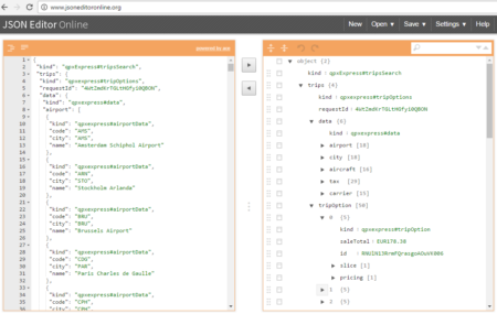
However, looking deeply into the object, several other elements are provided as the distance in mile, the segment, the duration, the carrier, etc. The R parser to transform the json structure in a usable dataframe requires the dplyr library for using the pipe operator (%>%) to streamline the code and make the parser more readable. Nevertheless, the library actually wrangling through the lines is tidyjson and its powerful functions:
- enter_object: enters and dives into a data object;
- gather_array: stacks a JSON array;
- spread_values: creates new columns from values assigning specific type (e.g. jstring, jnumber).
library(dplyr) # for pipe operator %>% and other dplyr functions
library(tidyjson) # https://cran.r-project.org/web/packages/tidyjson/vignettes/introduction-to-tidyjson.html
data_items <- datajson %>%
spread_values(kind = jstring("kind")) %>%
spread_values(trips.kind = jstring("trips","kind")) %>%
spread_values(trips.rid = jstring("trips","requestId")) %>%
enter_object("trips","tripOption") %>%
gather_array %>%
spread_values(
id = jstring("id"),
saleTotal = jstring("saleTotal")) %>%
enter_object("slice") %>%
gather_array %>%
spread_values(slice.kind = jstring("kind")) %>%
spread_values(slice.duration = jstring("duration")) %>%
enter_object("segment") %>%
gather_array %>%
spread_values(
segment.kind = jstring("kind"),
segment.duration = jnumber("duration"),
segment.id = jstring("id"),
segment.cabin = jstring("cabin")) %>%
enter_object("leg") %>%
gather_array %>%
spread_values(
segment.leg.aircraft = jstring("aircraft"),
segment.leg.origin = jstring("origin"),
segment.leg.destination = jstring("destination"),
segment.leg.mileage = jnumber("mileage")) %>%
select(kind, trips.kind, trips.rid,
saleTotal,id, slice.kind, slice.duration,
segment.kind, segment.duration, segment.id,
segment.cabin, segment.leg.aircraft, segment.leg.origin,
segment.leg.destination, segment.leg.mileage)
head(data_items)
kind trips.kind trips.rid saleTotal
1 qpxExpress#tripsSearch qpxexpress#tripOptions UnxCOx4nKIcIOpRiG0QBOe EUR178.38
2 qpxExpress#tripsSearch qpxexpress#tripOptions UnxCOx4nKIcIOpRiG0QBOe EUR178.38
3 qpxExpress#tripsSearch qpxexpress#tripOptions UnxCOx4nKIcIOpRiG0QBOe EUR235.20
4 qpxExpress#tripsSearch qpxexpress#tripOptions UnxCOx4nKIcIOpRiG0QBOe EUR235.20
5 qpxExpress#tripsSearch qpxexpress#tripOptions UnxCOx4nKIcIOpRiG0QBOe EUR248.60
6 qpxExpress#tripsSearch qpxexpress#tripOptions UnxCOx4nKIcIOpRiG0QBOe EUR248.60
id slice.kind slice.duration
1 ftm7QA6APQTQ4YVjeHrxLI006 qpxexpress#sliceInfo 510
2 ftm7QA6APQTQ4YVjeHrxLI006 qpxexpress#sliceInfo 510
3 ftm7QA6APQTQ4YVjeHrxLI009 qpxexpress#sliceInfo 490
4 ftm7QA6APQTQ4YVjeHrxLI009 qpxexpress#sliceInfo 490
5 ftm7QA6APQTQ4YVjeHrxLI007 qpxexpress#sliceInfo 355
6 ftm7QA6APQTQ4YVjeHrxLI007 qpxexpress#sliceInfo 355
segment.kind segment.duration segment.id segment.cabin
1 qpxexpress#segmentInfo 160 GixYrGFgbbe34NsI COACH
2 qpxexpress#segmentInfo 235 Gj1XVe-oYbTCLT5V COACH
3 qpxexpress#segmentInfo 190 Grt369Z0shJhZOUX COACH
4 qpxexpress#segmentInfo 155 GRvrptyoeTfrSqg8 COACH
5 qpxexpress#segmentInfo 100 GXzd3e5z7g-5CCjJ COACH
6 qpxexpress#segmentInfo 105 G8axcks1R8zJWKrN COACH
segment.leg.aircraft segment.leg.origin segment.leg.destination segment.leg.mileage
1 320 FCO IST 859
2 77W IST LHR 1561
3 73H FCO ARN 1256
4 73G ARN LHR 908
5 319 FCO STR 497
6 319 STR LHR 469
Data are now in an R-friendly structure despite not yet ready for analysis. As can be observed from the first rows, each record has information on a single
segment of the flight selected. A further step of aggregation using some SQL is needed in order to end up with a dataframe of flights data suitable for statistical analysis.
Next up, the aggregation, some
data analysis and
data visualization to complete the journey through the web data acquisition using R.
#R #rstats #maRche #json #curl #tidyjson #Rbloggers
This post is also shared in www.r-bloggers.com and LinkedIn