#json – R-posts.com

New DataCamp Course: Working with Web Data in R

Hi there! We just launched Working with Web Data in R by Oliver Keyes and Charlotte Wickham, our latest R course!

Most of the useful data in the world, from economic data to news content to geographic information, lives somewhere on the internet – and this course will teach you how to access it. You’ll explore how to work with APIs (computer-readable interfaces to websites), access data from Wikipedia and other sources, and build your own simple API client. For those occasions where APIs are not available, you’ll find out how to use R to scrape information out of web pages. In the process, you’ll learn how to get data out of even the most stubborn website, and how to turn it into a format ready for further analysis. The packages you’ll use and learn your way around are rvest, httr, xml2 and jsonlite, along with particular API client packages like WikipediR and pageviews.

Take me to chapter 1!

Working with Web Data in R features interactive exercises that combine high-quality video, in-browser coding, and gamification for an engaging learning experience that will make you an expert in getting information from the Internet!

What you’ll learn

1. Downloading Files and Using API Clients
Sometimes getting data off the internet is very, very simple – it’s stored in a format that R can handle and just lives on a server somewhere, or it’s in a more complex format and perhaps part of an API but there’s an R package designed to make using it a piece of cake. This chapter will explore how to download and read in static files, and how to use APIs when pre-existing clients are available.

2. Using httr to interact with APIs directly
If an API client doesn’t exist, it’s up to you to communicate directly with the API. But don’t worry, the package httr makes this really straightforward. In this chapter, you’ll learn how to make web requests from R, how to examine the responses you get back and some best practices for doing this in a responsible way.

3. Handling JSON and XML
Sometimes data is a TSV or nice plaintext output. Sometimes it’s XML and/or JSON. This chapter walks you through what JSON and XML are, how to convert them into R-like objects, and how to extract data from them. You’ll practice by examining the revision history for a Wikipedia article retrieved from the Wikipedia API using httr, xml2 and jsonlite.

4. Web scraping with XPATHs
Now that we’ve covered the low-hanging fruit (“it has an API, and a client”, “it has an API”) it’s time to talk about what to do when a website doesn’t have any access mechanisms at all – when you have to rely on web scraping. This chapter will introduce you to the rvest web-scraping package, and build on your previous knowledge of XML manipulation and XPATHs.

5. ECSS Web Scraping and Final Case Study
CSS path-based web scraping is a far-more-pleasant alternative to using XPATHs. You’ll start this chapter by learning about CSS, and how to leverage it for web scraping. Then, you’ll work through a final case study that combines everything you’ve learnt so far to write a function that queries an API, parses the response and returns data in a nice form.

Master web data in R with our course Working with Web Data in R!

Web data acquisition: from database to dataframe for data analysis and visualization (Part 4)

The previous post described how the deeply nested JSON data on fligths were parsed and stored in an R-friendly database structure. However, looking into the data, the information is not yet ready for statistical analysis and visualization and some further processing is necessary before extracting insights and producing nice plots. In the parsed batch, it is clearly visible the redundant structure of the data with the flight id repeted for each segment of each flight. This is also confirmed with the following simple check as the rows of the dataframe are more than the unique counts of the elements in the id column.

dim(data_items)
[1] 397  15

length(unique(data_items$id))
201

# real time changes of data could produce different results

This implies that the information of each segment of each flight has to be aggregated and merged in a dataset as single observations of a statistical analysis between, for example, price and distance. First, a unique primary key for each observation has to be used as reference variable to uniquely identify each element of the dataset.

library(plyr) # sql like functions
library(readr) # parse numbers from strings
 
data_items <- data.frame(data_items)
 
# id (primary key)
data <- data.frame(unique(data_items$id))
colnames(data) <- c('id')
 
# n° of segment
n_segment <- aggregate(data_items['segment.id'], by=data_items['id'], length)
data <- join(data, n_segment, by='id', type='left', match='first') # sql left join
# mileage
mileage <- aggregate(data_items['segment.leg.mileage'], by=data_items['id'], sum)
data <- join(data, mileage, by='id', type='left', match='first') # sql left join
# price
price <- data.frame('id'=data_items$id, 'price'=parse_number(data_items$saleTotal))
data <- join(data, price, by='id', type='left', match='first') # sql left join
# dataframe
colnames(data) <- c('id','segment', 'mileage', 'price')
head(data)

The aggregation of mileage and price using the unique primary key allows to set up a dataframe ready for statistical analysis and data visualization. Current data tells us that there is a maximum of three segments in the connection between FCO and LHR with a minimum price of around EUR 122 and a median around EUR 600.


# descriptive statistics
summary(data)
 
 
# histogram price & distance
g1 <- ggplot(data, aes(x=price)) + 
  geom_histogram(bins = 50) +  
  ylab("Distribution of the Price (EUR)") +
  xlab("Price (EUR)") 
 
g2 <- ggplot(data, aes(x=mileage)) + 
  geom_histogram(bins = 50) +  
  ylab("Distribution of the Distance") +
  xlab("Distance (miles)")
 
grid.arrange(g1, g2)
# price - distance relationship
s0 <- ggplot(data = data, aes(x = mileage, y = price)) +
    geom_smooth(method = "lm", se=FALSE, color="black") +
    geom_point() + labs(x = "Distance in miles", y = "Price (EUR)")
s0 <- ggMarginal(s0, type = "histogram", binwidth = 30)
s0

Of course, plenty of other analysis and graphical representations using flights features are possible given the large set of variables available in QPX Express API and the availability of data in real time.

To conclude the 4-step (flight) trip from data acquisition to data analysis, let's recap the most important concepts described in each of the post: 1) Client-Server connection 2) POST request in R 3) Data parsing and structuring 4) Data analysis and visualization

That's all folks! #R #rstats #maRche #json #curl #qpxexpress #Rbloggers This post is also shared in www.r-bloggers.com

Web data acquisition: parsing json objects with tidyjson (Part 3)

The collection of example flight data in json format available in part 2, described the libraries and the structure of the POST request necessary to collect data in a json object. Despite the process generated and transferred locally a proper response, the data collected were neither in a suitable structure for data analysis nor immediately readable. They appears as just a long string of information nested and separated according to the JavaScript object notation syntax. Thus, to visualize the deeply nested json object and make it human readable and understandable for further processing, the json content could be copied and pasted in a common online parser. The tool allows to select each node of the tree and observe the data structure up to the variables and data of interest for the statistical analysis. The bulk of the relevant information for the purpose of the analysis on flight prices are hidden in the tripOption node as shown in the following figure (only 50 flight solutions were requested).

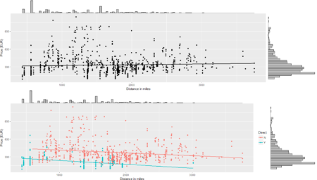
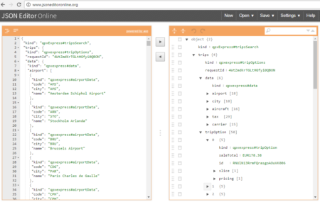
However, looking deeply into the object, several other elements are provided as the distance in mile, the segment, the duration, the carrier, etc. The R parser to transform the json structure in a usable dataframe requires the dplyr library for using the pipe operator (%>%) to streamline the code and make the parser more readable. Nevertheless, the library actually wrangling through the lines is tidyjson and its powerful functions:

enter_object: enters and dives into a data object;
gather_array: stacks a JSON array;
spread_values: creates new columns from values assigning specific type (e.g. jstring, jnumber).

library(dplyr) # for pipe operator %>% and other dplyr functions library(tidyjson) # https://cran.r-project.org/web/packages/tidyjson/vignettes/introduction-to-tidyjson.html data_items <- datajson %>% spread_values(kind = jstring("kind")) %>% spread_values(trips.kind = jstring("trips","kind")) %>% spread_values(trips.rid = jstring("trips","requestId")) %>% enter_object("trips","tripOption") %>% gather_array %>% spread_values( id = jstring("id"), saleTotal = jstring("saleTotal")) %>% enter_object("slice") %>% gather_array %>% spread_values(slice.kind = jstring("kind")) %>% spread_values(slice.duration = jstring("duration")) %>% enter_object("segment") %>% gather_array %>% spread_values( segment.kind = jstring("kind"), segment.duration = jnumber("duration"), segment.id = jstring("id"), segment.cabin = jstring("cabin")) %>% enter_object("leg") %>% gather_array %>% spread_values( segment.leg.aircraft = jstring("aircraft"), segment.leg.origin = jstring("origin"), segment.leg.destination = jstring("destination"), segment.leg.mileage = jnumber("mileage")) %>% select(kind, trips.kind, trips.rid, saleTotal,id, slice.kind, slice.duration, segment.kind, segment.duration, segment.id, segment.cabin, segment.leg.aircraft, segment.leg.origin, segment.leg.destination, segment.leg.mileage) head(data_items) kind trips.kind trips.rid saleTotal 1 qpxExpress#tripsSearch qpxexpress#tripOptions UnxCOx4nKIcIOpRiG0QBOe EUR178.38 2 qpxExpress#tripsSearch qpxexpress#tripOptions UnxCOx4nKIcIOpRiG0QBOe EUR178.38 3 qpxExpress#tripsSearch qpxexpress#tripOptions UnxCOx4nKIcIOpRiG0QBOe EUR235.20 4 qpxExpress#tripsSearch qpxexpress#tripOptions UnxCOx4nKIcIOpRiG0QBOe EUR235.20 5 qpxExpress#tripsSearch qpxexpress#tripOptions UnxCOx4nKIcIOpRiG0QBOe EUR248.60 6 qpxExpress#tripsSearch qpxexpress#tripOptions UnxCOx4nKIcIOpRiG0QBOe EUR248.60 id slice.kind slice.duration 1 ftm7QA6APQTQ4YVjeHrxLI006 qpxexpress#sliceInfo 510 2 ftm7QA6APQTQ4YVjeHrxLI006 qpxexpress#sliceInfo 510 3 ftm7QA6APQTQ4YVjeHrxLI009 qpxexpress#sliceInfo 490 4 ftm7QA6APQTQ4YVjeHrxLI009 qpxexpress#sliceInfo 490 5 ftm7QA6APQTQ4YVjeHrxLI007 qpxexpress#sliceInfo 355 6 ftm7QA6APQTQ4YVjeHrxLI007 qpxexpress#sliceInfo 355 segment.kind segment.duration segment.id segment.cabin 1 qpxexpress#segmentInfo 160 GixYrGFgbbe34NsI COACH 2 qpxexpress#segmentInfo 235 Gj1XVe-oYbTCLT5V COACH 3 qpxexpress#segmentInfo 190 Grt369Z0shJhZOUX COACH 4 qpxexpress#segmentInfo 155 GRvrptyoeTfrSqg8 COACH 5 qpxexpress#segmentInfo 100 GXzd3e5z7g-5CCjJ COACH 6 qpxexpress#segmentInfo 105 G8axcks1R8zJWKrN COACH segment.leg.aircraft segment.leg.origin segment.leg.destination segment.leg.mileage 1 320 FCO IST 859 2 77W IST LHR 1561 3 73H FCO ARN 1256 4 73G ARN LHR 908 5 319 FCO STR 497 6 319 STR LHR 469 Data are now in an R-friendly structure despite not yet ready for analysis. As can be observed from the first rows, each record has information on a single segment of the flight selected. A further step of aggregation using some SQL is needed in order to end up with a dataframe of flights data suitable for statistical analysis. Next up, the aggregation, some data analysis and data visualization to complete the journey through the web data acquisition using R. #R #rstats #maRche #json #curl #tidyjson #Rbloggers This post is also shared in www.r-bloggers.com and LinkedIn