Invitation to the 3rd Big Data Analytics World Championships 2017
We invite members of the R-Bloggers/R-Users community to participate in the 2017 TEXATA Big Data Analytics World Championships (www.texata.com).
You’re Free Discount Code is: 2017RUSERS (normally $30 fully paid entry).
Here are important dates for the TEXATA educational business competition:
Round 1 on 30th September 2017 (Online)Round 2 on14th October 2017 (Online)World Finals on15th-16th November 2017(Austin)About TEXATA
The competition is a celebration of big data analytics skills and communities. It targets at students and young professionals looking to learn more and showcase their creative business skills in big data analytics. It’s ideal for people working or studying or interested in: Technology, Computer Science, Statistics and Data, Data Science, IT Professionals, Software Engineering, Analytical, Quantitative and Engineering disciplines. The competition is a great way to learn more about leading Companies, Communities, Universities and Institutions in the big data and business analytics industries. All participants will receive updates throughout 2017 and 2018 of free offers, upcoming conferences and educational events of our community partners as part of joining the TEXATA event. Best of all, it’s all free with this discount code thanks to RBloggers/R-Users.
How It Works
The structure involves two Online Rounds with a Live World Finals in Austin Texas. Each of the Online Rounds will last 4 Hours in duration. The Top World Finalists will be flown from around the world to compete in the case-study based finals challenge with Finals Judges. The organizers hold similar world championship events in other professional services industries – including Finance and Financial Modeling (www.modeloff.com) and High IQ World Championships (www.hiqora.com) – which gives participants a good background idea of the nature of the educational, fun and challenging nature of the elite business and professional league competitions.
Visit www.texata.com for more information.
Principal Component Analysis (PCA) is a technique used to find the core components that underlie different variables. It comes in very useful whenever doubts arise about the true origin of three or more variables. There are two main methods for performing a PCA: naive or less naive. In the naive method, you first check some conditions in your data which will determine the essentials of the analysis. In the less-naive method, you set the those yourself, based on whatever prior information or purposes you had. I will tackle the naive method, mainly by following the guidelines inField, Miles, and Field (2012), with updated code where necessary. Thislecture materialwas also useful.
The ‘naive’ approach is characterized by a first stage that checks whether the PCA should actually be performed with your current variables, or if some should be removed. The variables that are accepted are taken to a second stage which identifies the number of principal components that seem to underlie your set of variables. I ascribe these to the ‘naive’ or formal approach because either or both could potentially be skipped in exceptional circumstances, where the purpose is not scientific, or where enough information exists in advance.
STAGE 1. Determine whether PCA is appropriate at all, considering the variables
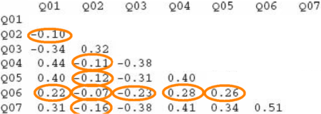
Variables should beinter-correlated enough but not too much.Field et al. (2012) provide some thresholds, suggesting that no variable should have many correlations below .30, oranycorrelation at all above .90. Thus, in the example here, variable Q06 should probably be excluded from the PCA.
Bartlett’s test, on the nature of the intercorrelations, should be significant. Significance suggests that the variables are not an ‘identity matrix’ in which correlations are a sampling error.
KMO(Kaiser-Meyer-Olkin), a measure of sampling adequacy based on common variance (so similar purpose as Bartlett’s). As Field et al. review, ‘values between .5 and .7 are mediocre, values between .7 and .8 are good, values between .8 and .9 are great and values above .9 are superb’ (p. 761). There’s a general score as well as one per variable. The general one will often be good, whereas the individual scores may more likely fail. Any variable with a score below .5 should probably be removed, and the test should be run again.
Determinant:A formula about multicollinearity. The result should preferably fall below .00001.
Note that some of these tests are run on the dataframe and others on a correlation matrix of the data, as distinguished below.
# Necessary libraries
library(ltm)
library(lattice)
library(psych)
library(car)
library(pastecs)
library(scales)
library(ggplot2)
library(arules)
library(plyr)
library(Rmisc)
library(GPArotation)
library(gdata)
library(MASS)
library(qpcR)
library(dplyr)
library(gtools)
library(Hmisc)
# Select only your variables of interest for the PCA
dataset = mydata[, c('select_var1','select_var1',
'select_var2','select_var3','select_var4',
'select_var5','select_var6','select_var7')]
# Create matrix: some tests will require it
data_matrix = cor(dataset, use = 'complete.obs')
# See intercorrelations
round(data_matrix, 2)
# Bartlett's
cortest.bartlett(dataset)
# KMO (Kaiser-Meyer-Olkin)
KMO(data_matrix)
# Determinant
det(data_matrix)
STAGE 2. Identify number of components (aka factors)
In this stage, principal components (formally called ‘factors’ at this stage) are identified among the set of variables.
The identification is done through a basic, ‘unrotated’ PCA. The number of components set a priori must equal the number of variables that are being tested.
# Start off with unrotated PCA
pc1 = psych::principal(dataset, nfactors =
length(dataset), rotate="none")
pc1
Below, an example result:
## Principal Components Analysis
## Call: psych::principal(r = eng_prop, nfactors = 3, rotate = "none")
## Standardized loadings (pattern matrix) based upon correlation matrix
## PC1 PC2 PC3 h2 u2 com
## Aud_eng -0.89 0.13 0.44 1 -2.2e-16 1.5
## Hap_eng 0.64 0.75 0.15 1 1.1e-16 2.0
## Vis_eng 0.81 -0.46 0.36 1 -4.4e-16 2.0
##
## PC1 PC2 PC3
## SS loadings 1.87 0.79 0.34
## Proportion Var 0.62 0.26 0.11
## Cumulative Var 0.62 0.89 1.00
## Proportion Explained 0.62 0.26 0.11
## Cumulative Proportion 0.62 0.89 1.00
##
## Mean item complexity = 1.9
## Test of the hypothesis that 3 components are sufficient.
##
## The root mean square of the residuals (RMSR) is 0
## with the empirical chi square 0 with prob < NA
##
## Fit based upon off diagonal values = 1
Among the columns, there are first the correlations between variables and components, followed by a column (h2) with the ‘communalities‘. If less factors than variables had been selected, communality values would be below 1. Then there is the uniqueness column (u2):uniquenessis equal to 1 minus the communality. Next is ‘com’, which reflects thecomplexitywith which a variable relates to the principal components. Those components are precisely found below. The first row contains the sums of squared loadings, or eigenvalues, namely, the total variance explained by each linear component. This value corresponds to the number of units explained out of all possible factors (which were three in the above example). The rows below all cut from the same cloth.Proportion var= variance explained over a total of 1. This is the result of dividing the eigenvalue by the number of components. Multiply by 100 and you get the percentage of total variance explained, which becomes useful. In the example, 99% of the variance has been explained. Aside from the meddling maths, we should actually expect 100% there because the number of factors equaled the number of variables.Cumulative var:variance added consecutively up to the last component.Proportion explained:variance explained over what has actually been explained (only when variables = factors is this the same as Proportion var).Cumulative proportion:the actually explained variance added consecutively up to the last component.
Two sources will determine the number of components to select for the next stage:
Kaiser’s criterion: components with SS loadings > 1. In our example, only PC1.
A more lenient alternative is Joliffe’s criterion, SS loadings > .7.
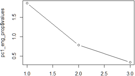
Scree plot:the number of points after point of inflexion. For this plot, call:
plot(pc1$values, type = 'b')
Imagine a straight linefrom the first point on the right.Once this line bends considerably, count the points after the bend and up to the last point on the left. The number of points is the number of components to select. The example here is probably the most complicated (two components were finally chosen), but normally it’snot difficult.
Based on both criteria, go ahead and select the definitive number of components.
STAGE 3. Run definitive PCA
Run a very similar command as you did before, but now with a more advanced method. The first PCA, a heuristic one, worked essentially on the inter-correlations. The definitive PCA, in contrast, will implement a prior shuffling known as ‘rotation’, to ensure that the result is robust enough (just like cards are shuffled). Explained variance is captured better this way. The go-to rotation method is the orthogonal, or ‘varimax’ (though others may be considered too).
# Now with varimax rotation, Kaiser-normalized
# by default:
pc2 = psych::principal(dataset, nfactors=2,
rotate = "varimax", scores = TRUE)
pc2
pc2$loadings
# Healthcheck
pc2$residual
pc2$fit
pc2$communality
We would want:
Less than half ofresidualswith absolute values > 0.05
Modelfit> .9
Allcommunalities> .7
If any of this fails, consider changing the number of factors. Next, the rotated components that have been ‘extracted’ from the core of the set of variables can be added to the dataset. This would enable the use of these components as new variables that might prove powerful and useful (as inthis research).
STAGE 4. Determine ascription of each variable to components
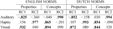
Check the main summary by just calling pc2, and see how each variable correlates with the rotated components. This is essential because it reveals how variables load on each component, or in other words, to which component a variable belongs. For instance, the table shown here belongs to a study about meaning of words. These results suggest that the visual and haptic modalities of words are quite related, whereas the auditory modality is relatively unique. When the analysis works out well, a cut-off point of r = .8 may be applied for considering a variable as part of a component.
STAGE 5. Enjoy the plot
The plot is perhaps the coolest part about PCA. It really makes an awesome illustration of the power of data analysis.
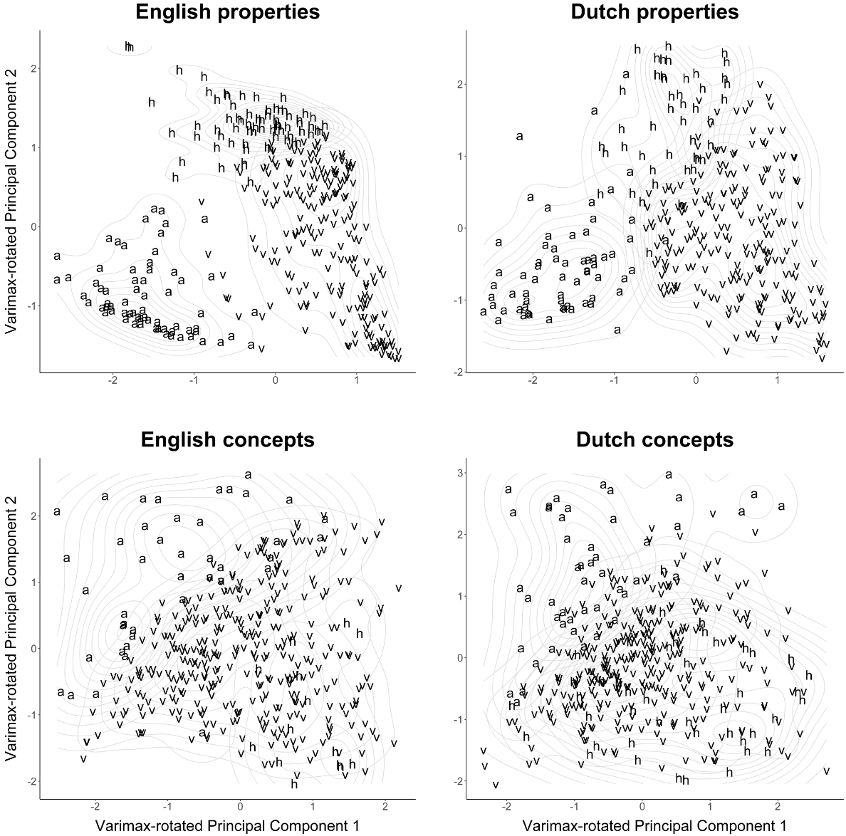
Below is an example combining PCA plots with code similar to the above. These plots illustrate something further with regard to the relationships among modalities. In property words, the different modalities spread out more clearly than they do in concept words. This makes sense because in language, properties define concepts (see more).
An example of this code is use isavailable here(withdata here).
References
Field, A. P., Miles, J., & Field, Z. (2012). Discovering statistics using R. London: Sage.
Feel free to comment below or on the original post.
Register now for ODSC West in San Francisco, November 2-4 and save 60% with code RB60 until September 1st.
R continues to hold its own in the data science landscape thanks in no small part to its flexibility. That flexibility allows R to integrate with some of the most popular data science tools available.
Given R’s memory bounds, it’s no surprise that deep learning tools like Tensorflow are on that list. Comprehensive, intuitive, and well documented, Tensorflow has quickly become one of the most popular deep learning platforms and RStudio released a package to integrate with the Tensorflow API. Not to be outdone MXNet, another popular and powerful deep learning framework has native support for R with an API interface.
It doesn’t stop with deep learning. Data science is moving real-time and the streaming analytics platform, Apache Kafka, is rapidly gaining traction with the community. The kafka package allows one to use the Kafka messaging queue via R. Spark is now one of the dominant machine learning platforms and thus we see multiple R integrations in the form of the spark package and the SparkR package. The list will continue to grow with package integrations released for H20.ai, Druid etc. and more on the way.
At the Open Data Science Conference, R has long been one of the most popular data science languages and ODSC West 2017 is no exception. We have a strong lineup this year that includes:
R Tools for Data Science
Modeling Big Data with R, sparklyr, and Apache Spark
Machine Learning with R
Introduction to Data Science with R
Modern Time-Series with Prophet
R4ML: A Scalable and Distributed framework in R for Machine Learning
Databases Using R
Geo-Spatial Data Visualization using R
From an R user perspective, one of the most exciting things about ODSC West 2017 is that it offers an excellent opportunity to do a deep dive into some of the most popular data science tools you can now leverage with R. Talks and workshops on the conference schedule include:
Deep learning from Scratch WIth Tensorflow
Apache Kafka for Real-time analytics
Deep learning with MXNet
Effective TensorFlow
Building an Open Source Analytics Solution with Kafka and Druid
Deep Neural Networks with Keras
Robust Data Pipelines with Apache Airflow
Apache Superset – A Modern, Enterprise-Ready Business Intelligence Web Application
Over 3 packed days, ODSC West 2017 also offers a great opportunity to brush up on your modeling skills that include predictive analytics, time series, NLP, machine learning, image recognition, deep learning. autonomous vehicles, and AI chatbot assistants. Here’s just a few of the data science workshops and talks scheduled:
Feature Selection from High Dimensions
Interpreting Predictions from Complex Models
Deep Learning for Recommender Systems
Natural Language Processing in Practice – Do’s and Don’ts
Machine Imaging recognition
Training a Prosocial Chatbot
Anomaly Detection Using Deep Learning
Myths of Data Science: Practical Issues You Can and Can Not Ignore.
Playing Detective with CNNs
Recommendation System Architecture and Algorithms
Driver and Occupants Monitoring AI for Autonomous Vehicles
Solving Impossible Problems by Collaborating with an AI
Dynamic Risk Networks: Mapping Risk in the Financial System
With over 20 full training session, 50 workshops and 100 speakers, ODSC West 2017 is ideal for beginners to experts looking to understand the latest in R tools and topics in data science and AI.
Register now and save 60% with code RB60 until September 1st.
Lately I’ve been working a lot with the shinydashboard library.
Like shiny, it allows any R programmer to harness the power of R and create professional looking interactive apps. The thing about shinydashboards is that it makes wonderfully looking dashboards.
What I’ve been doing with the dashboards is to create dedicated dashboards for my customers. Since most of my customers speak, read, and write in Hebrew I needed to fit that into my shinydashboard apps (i.e., fully localize the app). See an example for such a localized dashboard I made here.
Making a shinydashboard localized turned out to be simpler than I thought.
Since the average R programmer doesn’t necessarily know and understand CSS, I thought I post my solution. This should fit any Hebrew or Arabic dashboard to work from right to left, including the sidebar and all other objects (though I only tested it in Hebrew).
If you want the short version:
(1) Download the following css file;
(2) Put it in a subfolder “/www” of your shinydashboard app;
(3) In your dashboardBody command (within the ui.R section of your shiny app) add the following code: dashboardBody(
tags$head(
tags$link(rel = "stylesheet", type = "text/css", href = "bootstrap-rtl.css"
),...
Here are the few insights and steps which lead me to this solution:
Insight #1: any shiny app (dashboard or otherwise) can be customized using CSS. That’s no secret. However, the adaptation to RTL isn’t that simple when you have so many objects, mobile responsiveness to worry about, etc.
Insight #2: Shiny is based on the AdminLTE theme which is based on the bootstrap 3 theme. AdminLTE is a great theme, and even though it doesn’t officially support RTL, mmdsharifi, provided a solution in his github page. The same for bootstrap 3 which has an RTL customization by morteza (also on github).
Insight #3: What I did in order to make this work was to take the bootstrap-rtl.css from morteza, and then concatenate the AdminLTE-rtl.css file by mmdsharifi. Voilà! (simple, isn’t it?)
K-Means Clustering is a well known technique based on unsupervised learning. As the name mentions, it forms ‘K’ clusters over the data using mean of the data. Unsupervised algorithms are a class of algorithms one should tread on carefully. Using the wrong algorithm will give completely botched up results and all the effort will go down the drain. Unlike supervised learning algorithms where one can still get around keeping some parts as an unknown black box, knowing the technique inside out starting from the assumptions made to the process, methods of optimization and uses is essential. So let us begin step by step starting from the assumptions. I will then explain the process and a hands-on illustration using
Assumptions and Process Why do we assume in the first place? The answer is that making assumptions helps simplify problems and simplified problems can then be solved accurately. To divide your dataset into clusters, one must define the criteria of a cluster and those make the assumptions for the technique. K-Means clustering method considers two assumptions regarding the clusters – first that the clusters are spherical and second that the clusters are of similar size. Spherical assumption helps in separating the clusters when the algorithm works on the data and forms clusters. If this assumption is violated, the clusters formed may not be what one expects. On the other hand, assumption over the size of clusters helps in deciding the boundaries of the cluster. This assumption helps in calculating the number of data points each cluster should have. This assumption also gives an advantage. Clusters in K-means are defined by taking the mean of all the data points in the cluster. With this assumption, one can start with the centers of clusters anywhere. Keeping the starting points of the clusters anywhere will still make the algorithm converge with the same final clusters as keeping the centers as far apart as possible.
Now let’s understand how the algorithm works. The first step is to assign initial clusters. You can specify any K clusters or let the algorithm assign them randomly. The algorithm works in iterations and in every iteration, all the data points are then assigned to one of the clusters based on the nearest distance from the centers. After all points are assigned to one of the cluster, the cluster centers are now updated. The new centers are decided based on the centroid mean of all the points within the cluster. This is repeated, iteration after iteration until the there is no change in the cluster assignment of any of the data points but there are a lot of calculations which are not fixed in this algorithm. For example, one can decide how the distance for each data point from the cluster center is defined. All of us are familiar with the Euclidean distance. The algorithm is straightforward and easy to understand but using the technique is not as easy as it looks. Let’s try out some examples in R.
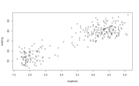
K-Means Starter To understand how K-Means works, we start with an example where all our assumptions hold. R includes a dataset about waiting time between eruptions and the duration of the eruption for the Old Faithful geyser in Yellowstone National Park known as ‘faithful’. The dataset consists of 272 observations of 2 features.
#Viewing the Faithful dataset
plot(faithful)
Looking at the dataset, we can notice two clusters. I will now use the kmeans() function in R to form clusters. Let’s see how K-Means clustering works on the data
#Specify 2 centers
k_clust_start=kmeans(faithful, centers=2)
#Plot the data using clusters
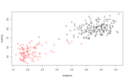
plot(faithful, col=k_clust_start$cluster,pch=2)
Being a small dataset, clusters are formed almost instantaneously but how do we see the clusters, their centers or sizes? The k_clust_start variable I used contains information on both centers and the size of clusters. Let’s check them out
#Use the centers to find the cluster centers
k_clust_start$centers
eruptions waiting
1 4.29793 80.28488
2 2.09433 54.75000
#Use the size to find the cluster sizes
k_clust_start$size
[1] 172 100
This means the first cluster consists of 172 members and is centered at 4.29793 value of eruptions and 80.28488 value of waiting. Similarly the second cluster consists of 100 members with 2.09433 value of eruptions and 54.75 value of waiting. Now this information is golden! We know that these centers are the cluster means. So, the eruptions typically happen for either ~2 mins or ~4.3 mins. For longer eruptions, the waiting time is also longer.
Getting into the depths Imagine a dataset which has clusters which one can clearly identify but k-means cannot. I’m talking about a dataset which does not satisfy the assumptions. A common example is a dataset which represents two concentric circles. Let’s generate it and see how it looks like
#The following code will generate different plots for you but they will be similar
library(plyr)
library(dplyr)
#Generate random data which will be first cluster
clust1 = data_frame(x = rnorm(200), y = rnorm(200))
#Generate the second cluster which will ‘surround’ the first cluster
clust2 =data_frame(r = rnorm(200, 15, .5), theta = runif(200, 0, 2 * pi),
x = r * cos(theta), y = r * sin(theta)) %>%
dplyr::select(x, y)
#Combine the data
dataset_cir= rbind(clust1, clust2)
#see the plot
plot(dataset_cir)
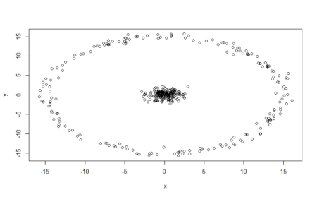
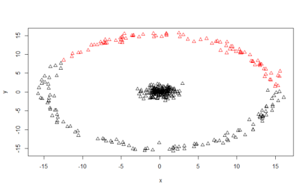
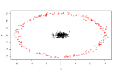
Simple, isn’t it? There are two clusters – one in the middle and the other circling the first. However, this violates the assumption that the clusters are spherical. The inner data is spherical while the outer circle is not. Even though the clustering will not be good, let’s see how does k-means perform on this data
#Fit the k-means model
k_clust_spher1=kmeans(dataset_cir, centers=2)
#Plot the data and clusters
plot(dataset_cir, col=k_clust_spher1$cluster,pch=2)
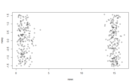
How do we solve this problem? There are clearly 2 clusters but k-means is not working well. A simple way in this case is to transform our data into polar format. Let’s convert it and plot it.
#Using a function for transformation
cart2pol=function(x,y){
#This is r
newx=sqrt(x^2 + y^2)
#This is theta
newy=atan(y/x)
x_y=cbind(newx,newy)
return(x_y)
}
dataset_cir2=cart2pol(dataset_cir$x,dataset_cir$y)
plot(dataset_cir2)
Now we run the k-means model on this data
k_clust_spher2=kmeans(dataset_cir2, centers=2)
#Plot the data and clusters
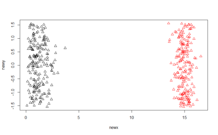
plot(dataset_cir2, col=k_clust_spher2$cluster,pch=2)
This time k-means algorithm works well and correctly transform the data. We can also view the clusters on the original data to double-check this.
By transforming our data into polar coordinates and fitting k-means model on the transformed data, we fulfil the spherical data assumption and data is accurately clustered. Now let’s look at a data where the clusters are not of similar sizes. Similar size does not mean that the clusters have to be exactly equal. It simply means that no cluster should have ‘too few’ members.
#Make the first cluster with 1000 random values
clust1 = data_frame(x = rnorm(1000), y = rnorm(1000))
#Keep 10 values together to make the second cluster
clust2=data_frame(x=c(5,5.1,5.2,5.3,5.4,5,5.1,5.2,5.3,5.4),y=c(5,5,5,5,5,4.9,4.9,4.9,4.9,4.9))
#Combine the data
dataset_uneven=rbind(clust1,clust2)
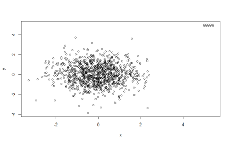
plot(dataset_uneven)
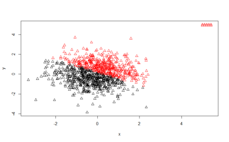
Here again, we have two clear clusters but they do not satisfy similar size requirement of k-means algorithm.
Why did this happen? K-means tries to minimize inter cluster and intracluster distance and create ‘tight’ clusters. In this process, it assigns some data points in the first cluster to the second cluster incorrectly. This makes the clustering inaccurate.
How to decide the value of K in data
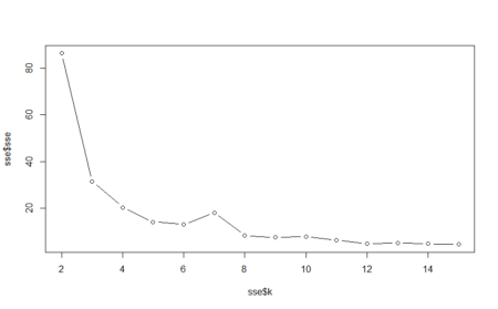
The datasets I worked on in this article are all simple and it is easily to identify clusters by plotting them. However, complicated datasets do not have this luxury. The Elbow method is popular for finding a suitable value of ‘K’ for k-means clustering. This method uses SSE within groups for different values of k and plots them. Using this plot, we can choose the ‘k’ which shows an abrupt change in SSE, creating an ‘elbow effect’. I will show an illustration on iris dataset using petal width and petal length.
#Create a vector for storing the sse
sse=vector('numeric')
for(i in 2:15){
#k-means function in R has a feature withinss which stores sse for each cluster group
sse[i-1]=sum(kmeans(iris[,3:4],centers=i)$withinss)
}
#Converting the sse to a data frame and storing corresponding value of k
sse=as.data.frame(sse)
sse$k=seq.int(2,15)
#Making the plot. This plot is also known as screeplot
plot(sse$k,sse$sse,type="b")
In this plot, the first elbow is formed at k=3. This method suggest that we should have 3 clusters for this data.
Conclusion
K-means clustering is one of the first and most basic clustering techniques whenever one thinks of unsupervised clustering. However, this technique is not just powerful, but also teaches the importance of understanding the data in unsupervised learning. If any of the assumptions are violated then the clusters are not formed properly. Similarly, while determining the value of ‘k’, using improper or arbitrary values may lead to improper clusters. In a way, k-means clustering also relies on the correct value of k for clustering the data accurately. Unsupervised learning is fun but not a wild attempt. One must be clear of all aspects of the algorithm and its assumptions before implementing it rather than treating it as a black box and shooting in the dark. This article illustrates the various shortcomings of improperly clustering data on simple datasets which do not satisfy the assumptions of the algorithm. The full code used in this article is given below.
#Viewing the Faithful dataset
plot(faithful)
#Specify 2 centers
k_clust_start=kmeans(faithful, centers=2)
#Plot the data using clusters
plot(faithful, col=k_clust_start$cluster,pch=2)
#Use the centers to find the cluster centers
k_clust_start$centers
#Use the size to find the cluster sizes
k_clust_start$size
#The following code will generate different plots for you but they will be similar
library(plyr)
library(dplyr)
#Generate random data which will be first cluster
clust1 = data_frame(x = rnorm(200), y = rnorm(200))
#Generate the second cluster which will ‘surround’ the first cluster
clust2 =data_frame(r = rnorm(200, 15, .5), theta = runif(200, 0, 2 * pi),
x = r * cos(theta), y = r * sin(theta)) %>%
dplyr::select(x, y)
#Combine the data
dataset_cir= rbind(clust1, clust2)
#see the plot
plot(dataset_cir)
#Fit the k-means model
k_clust_spher1=kmeans(dataset_cir, centers=2)
#Plot the data and clusters
plot(dataset_cir, col=k_clust_spher1$cluster,pch=2)
#Using a function for transformation
cart2pol=function(x,y){
#This is r
newx=sqrt(x^2 + y^2)
#This is theta
newy=atan(y/x)
x_y=cbind(newx,newy)
return(x_y)
}
dataset_cir2=cart2pol(dataset_cir$x,dataset_cir$y)
plot(dataset_cir2)
k_clust_spher2=kmeans(dataset_cir2, centers=2)
#Plot the data and clusters
plot(dataset_cir2, col=k_clust_spher2$cluster,pch=2)
plot(dataset_cir, col=k_clust_spher2$cluster,pch=2)
#Make the first cluster with 1000 random values
clust1 = data_frame(x = rnorm(1000), y = rnorm(1000))
#Keep 10 values together to make the second cluster
clust2=data_frame(x=c(5,5.1,5.2,5.3,5.4,5,5.1,5.2,5.3,5.4),y=c(5,5,5,5,5,4.9,4.9,4.9,4.9,4.9))
#Combine the data
dataset_uneven=rbind(clust1,clust2)
plot(dataset_uneven)
k_clust_spher3=kmeans(dataset_uneven, centers=2)
plot(dataset_uneven, col=k_clust_spher3$cluster,pch=2)
#Create a vector for storing the sse
sse=vector('numeric')
for(i in 2:15){
#k-means function in R has a feature withinss which stores sse for each cluster group
sse[i-1]=sum(kmeans(iris[,3:4],centers=i)$withinss)
}
#Converting the sse to a data frame and storing corresponding value of k
sse=as.data.frame(sse)
sse$k=seq.int(2,15)
#Making the plot. This plot is also known as scree-plot
plot(sse$k,sse$sse,type="b")
Bio: Chaitanya Sagar is the Founder and CEO of Perceptive Analytics. Perceptive Analytics has been chosen as one of the top 10 analytics companies to watch out for by Analytics India Magazine. It works on Marketing Analytics for e-commerce, Retail and Pharma companies.
If something takes less time if done through parallel processing, why not do it and save time? Modern laptops and PCs today have multi core processors with sufficient amount of memory available and one can use it to generate outputs quickly. Parallelizing your codes has its own numerous advantages. Instead of waiting several minutes or hours while a task completes, one can replace the code, obtain output within seconds or minutes and make it efficient at the same time. Code efficiency is one of the most sought abilities in the industry today and not many people are able to use it. Once you learn, how to parallelize your code, you will only regret that why didn’t you learn it sooner.
Parallelizing your codes in R is simple and there are various methods and packages. Let’s look at some of the functions available in R
lapply() and sapply() functions
lapply() function is used to apply a specified function to the vector or list input. The output of this function is always a list.
lapply(1:5, function(x) x^2)
#input is 1,2,3,4,5 and output is square of the input
[[1]]
[1] 1
[[2]]
[1] 4
[[3]]
[1] 9
[[4]]
[1] 16
[[5]]
[1] 25
We can also generate multiple outputs, say x^2 and x^3
lapply(1:5, function(x) c(x^2,x^3))
#The output should be square and cube of input
[[1]]
[1] 1 1
[[2]]
[1] 4 8
[[3]]
[1] 9 27
[[4]]
[1] 16 64
[[5]]
[1] 25 125
This output is very large but sometimes list is useful.
An alternative is to use the sapply() function which generates a vector, matrix or array output.
sapply(1:5, function(x) x^2) #This output is a vector
[1] 1 4 9 16 25
sapply(1:5, function(x) c(x^2,x^3)) #This outputs a matrix
[,1] [,2] [,3] [,4] [,5]
[1,] 1 4 9 16 25
[2,] 1 8 27 64 125
sapply() also provides two additional parameters: simplify and USE.NAMES. If both of them are kept false, the output generated is the same as lappy()
sapply(1:5, function(x) x^2, simplify = FALSE, USE.NAMES = FALSE)
#Output is same as for lapply()
[[1]]
[1] 1 1
[[2]]
[1] 4 8
[[3]]
[1] 9 27
[[4]]
[1] 16 64
[[5]]
[1] 25 125
The lapply() and sapply() functions are very fast in calculation. This means that the values are calculated independently of each other. However, it is not parallel in execution. There are various packages in R which allow parallelization.
“parallel” Package
The parallel package in R can perform tasks in parallel by providing the ability to allocate cores to R. The working involves finding the number of cores in the system and allocating all of them or a subset to make a cluster. We can then use the parallel version of various functions and run them by passing the cluster as an additional argument. A word of caution: it is important to close the cluster at the end of execution step so that core memory is released.
#Include the parallel library. If the next line does not work, run install.packages(“parallel”) first
library(parallel)
# Use the detectCores() function to find the number of cores in system
no_cores <- detectCores()
# Setup cluster
clust <- makeCluster(no_cores) #This line will take time
#The parallel version of lapply() is parLapply() and needs an additional cluster argument.
parLapply(clust,1:5, function(x) c(x^2,x^3))
[[1]]
[1] 1 1
[[2]]
[1] 4 8
[[3]]
[1] 9 27
[[4]]
[1] 16 64
[[5]]
[1] 25 125
stopCluster(clust)
If we want a similar output but with sapply(), we use the parSapply() function
#Include the parallel library. If the next line does not work, run install.packages(“parallel”) first
library(parallel)
# Use the detectCores() function to find the number of cores in system
no_cores <- detectCores()
# Setup cluster
clust <- makeCluster(no_cores) #This line will take time
#Setting a base variable
base <- 4
#Note that this line is required so that all cores in cluster have this variable available
clusterExport(clust, "base")
#Using the parSapply() function
parSapply(clust, 1:5, function(exponent) base^exponent)
[1] 4 16 64 256 1024
stopCluster(clust)
Notice the clusterExport() function here above? This is a special command needed to change the variable scope in parallel execution. Normally, variables such as ‘base’ have a scope which does not allow them to be accessible at all cores. We need to use the clusterExport() function and send the variable to all the assigned cores in the cluster. This is why we pass both the cluster variable as well as the variable we need to export. Changing the base variable after export will have no effect as all the cores will not see that change. Just like there is a scope for variables, libraries also need to be exported to all cores in order to be accessible. If I need to run a task which requires importing libraries, I use the
clusterEvalQ() function
clusterEvalQ(clust,library(randomForest))
“foreach” Package
Having basic programming knowledge makes you aware of for loops and the for each package is based on this methodology, making it easy to use. The foreach package also need doParallel package to make the process parallel using the registerDoParallel() function. The starting code looks like this
Once this is done, I can execute commands using the foreach() function and do them in parallel using the %dopar% command. The foreach() function includes a parameter .combine which is used to specify the kind of output needed. Using .combine=c gives a vector output while .combine=rbind creates a matrix. If a list output is needed similar to lapply(), we can set .combine=list. We can also obtain dataframe using .combine=data.frame
There are a number of different ways to do the same tasks which I did in the code above. For instance, the registerDoParallel() function allows creation of implicit clusters and we don’t need to use the makeCluster() function inside.
#This also works
registerDoParallel(no_cores)
Using implicit cluster means that I don’t have a ‘clust’ variable. To close the cluster, I need a different function known as stopImplicitCluster() at the end of our parallelization task.
stopImplicitCluster()
The foreach() and doParallel() functions have the local variables available at all cores by default. Hence, we don’t need any clusterExport function. However, variables which are not defined locally (such as those part of a parent function) and libraries need to be exported to all cores. For this, we have .export parameter and .packages parameter in foreach() function.
#using .export parameter
registerDoParallel(no_cores)
base <- 2 #Declaring this variable outside the scope of foreach() function
sample_func <- function (exponent) {
#Using the .export function here to include the base variable
foreach(exponent = 1:5, .combine = c,.export = "base") %dopar% base^exponent
}
sample_func()
[1] 2 4 8 16 32
stopImplicitCluster()
#using .packages parameter
library(dplyr)
registerDoParallel(no_cores)
foreach(i = 1:5, .combine=c, .packages="dplyr") %dopar% {
iris[i, ] %>% select(-Species) %>% sum
}
[1] 10.2 9.5 9.4 9.4 10.2
stopImplicitCluster()
With parallel processing comes efficient memory usage or your system may crash. The first thing that comes to mind is the ability to use same address(using FORK) versus creating different memory locations(using PSOCK). By default, the makeCluster() function creates addresses of type PSOCK. However, we can change the setting to FORK by passing the type function
clust<-makeCluster(no_cores, type="FORK")
Unless required, it is very useful to use the FORK type cluster to save memory and running time. The makeCluster() function also has an outfile parameter to specify an output file for debugging purpose.
starting worker pid=6696 on localhost:11363 at 17:34:36.808
starting worker pid=13168 on localhost:11363 at 17:34:37.421
starting worker pid=11536 on localhost:11363 at 17:34:38.047
starting worker pid=9572 on localhost:11363 at 17:34:38.675
starting worker pid=10612 on localhost:11363 at 17:34:43.467
starting worker pid=8864 on localhost:11363 at 17:34:44.078
starting worker pid=5144 on localhost:11363 at 17:34:44.683
starting worker pid=12012 on localhost:11363 at 17:34:45.286
[1] 1 2a" 3 4 5
We notice that a is printed after 2 in my output due to race. Using a different debug file for each node in a cluster is a better debugging option.
registerDoParallel(makeCluster(no_cores, outfile="debug_file.txt"))
foreach(x=list(1,2,3,4,5, "a")) %dopar% cat(dput(x), file = paste0("debug_file_", x, ".txt"))
In this case, I create 6 files containing output for each element in the list and a debug_file. Another way to debug code is using the trycatch() functions.
registerDoParallel(makeCluster(no_cores))
foreach(x=list(1, 2, "a")) %dopar%
{
tryCatch({
c(1/x) #Should give an error when x is “a”
}, error = function(e) return(paste0("Error occurred for '", x, "'",
" The error is '", e, "'")))
}
[[1]]
[1] 1
[[2]]
[1] 0.5
[[3]]
[1] "Error occurred for 'a' The error is 'Error in 1/x: non-numeric argument to binary operator\n'"
Debugging helps find out the reasons for errors but what if the error is related to running out of memory. For this, I can use rm() and gc() functions in R. The rm() function is used to remove a variable from the environment. If you’re sure that you no longer need this variable, it is better to free up memory using the rm() function.
base=4 #Create a variable base whose value is 4
base_copy=base #Make a copy of the variable
rm(base) #I can now remove the base variable and free up memory
To clean up the entire environment, use rm(list=ls()). It removes all the variables but does not remove libraries.
rm(list=ls())
The gc() function is the garbage collector for R and is automatically implemented. However, in a parallel environment, the gc() function is useful to return the memory regularly.
Summary
Parallel programming may seem a complex process at first but the amount of time saved after executing tasks in parallel makes it worth the try. Functions such as lapply() and sapply() are great alternatives to time consuming looping functions while parallel, foreach and doParallel packages are great starting points to running tasks in parallel. These parallel processes are based on functions and are also modular. However, with great power comes a risk of code crashes. Hence it is necessary to be careful and be aware of ways to control memory usage and error handling. It is not necessary to parallelize every piece of code that you write. You can always write sequential code and decide to parallelize the parts which take significant amounts of time. This will help in further reducing out of memory instances and writing robust and fast codes. The use of parallel programing method is growing and many packages now have parallel implementations available. With this article. one can dive deep into the world of parallel programming and make full use of the vast memory and processing power to generate output quickly. The full code for this article is as follows.
lapply(1:5, function(x) x^2) #input is 1,2,3,4,5 and output is square of the input
lapply(1:5, function(x) c(x^2,x^3)) #The output should be square and cube of input
sapply(1:5, function(x) x^2) #This output is a vector
sapply(1:5, function(x) c(x^2,x^3)) #This outputs a matrix
sapply(1:5, function(x) x^2, simplify = FALSE, USE.NAMES = FALSE) #Output is same as for lapply()
#Include the parallel library. If the next line does not work, run install.packages(“parallel”) first
library(parallel)
# Use the detectCores() function to find the number of cores in system
no_cores <- detectCores()
# Setup cluster
clust <- makeCluster(no_cores) #This line will take time
#The parallel version of lapply() is parLapply() and needs an additional cluster argument.
parLapply(clust,1:5, function(x) c(x^2,x^3))
stopCluster(clust)
#Include the parallel library. If the next line does not work, run install.packages(“parallel”) first
library(parallel)
# Use the detectCores() function to find the number of cores in system
no_cores <- detectCores()
# Setup cluster
clust <- makeCluster(no_cores) #This line will take time
#Setting a base variable
base <- 4
#Note that this line is required so that all cores in cluster have this variable available
clusterExport(clust, "base")
#Using the parSapply() function
parSapply(clust, 1:5, function(exponent) base^exponent)
stopCluster(clust)
clusterEvalQ(clust,library(randomForest))
library(foreach)
library(doParallel)
registerDoParallel(makeCluster(no_cores))
#Vector output
foreach(exponent = 1:5, .combine = c) %dopar% base^exponent
#Matrix output
foreach(exponent = 1:5, .combine = rbind) %dopar% base^exponent
#List output
foreach(exponent = 1:5, .combine = list, .multicombine=TRUE) %dopar% base^exponent
#Data Frame output
foreach(exponent = 1:5, .combine = data.frame) %dopar% base^exponent
#This also works
registerDoParallel(no_cores)
stopImplicitCluster()
#using .export parameter
registerDoParallel(no_cores)
base <- 2 #Declaring this variable outside the scope of foreach() function
sample_func <- function (exponent) {
#Using the .export function here to include the base variable
foreach(exponent = 1:5, .combine = c,.export = "base") %dopar% base^exponent
}
sample_func()
stopImplicitCluster()
#using .packages parameter
library(dplyr)
registerDoParallel(no_cores)
foreach(i = 1:5, .combine=c, .packages="dplyr") %dopar% {
iris[i, ] %>% select(-Species) %>% sum
}
stopImplicitCluster()
clust<-makeCluster(no_cores, type="FORK")
registerDoParallel(makeCluster(no_cores, outfile="debug_file.txt"))
foreach(x=list(1:5, "a")) %dopar% print(x)
registerDoParallel(makeCluster(no_cores, outfile="debug_file.txt"))
foreach(x=list(1,2,3,4,5, "a")) %dopar% cat(dput(x), file = paste0("debug_file_", x, ".txt"))
registerDoParallel(makeCluster(no_cores))
foreach(x=list(1, 2, "a")) %dopar%
{
tryCatch({
c(1/x) #Should give an error when x is “a”
}, error = function(e) return(paste0("Error occurred for '", x, "'",
" The error is '", e, "'")))
}
base=4 #Create a variable base whose value is 4
base_copy=base #Make a copy of the variable
rm(base) #I can now remove the base variable and free up memory
rm(list=ls())
Bio: Chaitanya Sagar is the Founder and CEO of Perceptive Analytics. Perceptive Analytics has been chosen as one of the top 10 analytics companies to watch out for by Analytics India Magazine. It works on Marketing Analytics for e-commerce, Retail and Pharma companies.
Adi Sarid (Tel Aviv university and Sarid Research Institute LTD.)
July-2017
Background
A while back I participated in an R workshop, in the annual convention of the Israeli Association for Statistics. I had the pleasure of talking with Tal Galili and Jonathan Rosenblatt which indicated that a lot of Israeli R users run into difficulties with Hebrew with R.
My firm opinion is that its best to keep everything in English, but sometimes you simply don’t have a choice. For example, I had to prepare a number of R shiny dashboards to Hebrew speaking clients, hence Hebrew was the way to go, in a kind of English-Hebrew “Mishmash” (mix).
I happened to run into a lot of such difficulties in the past, so here are a few pointers to get you started when working in R with Hebrew.
This post deals with Reading and writing files which contain Hebrew characters.
Note, there is also a bit to talk about in the context of Shiny apps which contain Hebrew and using right-to-left in shiny apps, and using Hebrew variable names. Both work with some care, but I won’t cover them here.
If you have any other questions you’d like to see answered, feel free to contact me [email protected].
Reading and writing files with Hebrew characters
R can read and write files in many formats. The common formats for small to medium data sets include the comma separated values (*.csv), and excel files (*.xlsx, *.xls). Each such read/write action is facilitated using some kind of “encoding”. Encoding, in simple terms, is a definition of a character set which help you operating system to interpret and represent the character as it should (לדוגמה, תווים בעברית). There are a number of relevant character sets (encodings) when Hebrew is concerned:
UTF-8
ISO 8859-8
Windows-1255
When you try to read files in which there are Hebrew characters, I usually recommend trying to read them in that order- UTF-8 is commonly used by a lot of applications, since it covers a lot of languages.
Using csv files with Hebrew characters
Here’s an example for something that can go wrong, and a possible solution. In this case I’ve prepared a csv file which encoded with UTF-8. When using R’s standard read.csv function, this is what happens:
## X.U.FEFF.שם גיל מגורים
## 1 רוני 25 חיפה
## 2 מוטי 77 הרצליה
## 3 דני 13 תל-אביב יפו
## 4 רעות 30 קרית שמונה
## 5 דנה 44 בית שאן
A bit better isn’t it? However, not perfect. We can read the Hebrew, but there is a weird thing in the header “X.U.FEFF”.
A better way to read and write files (much more than just encoding aspects – it’s quicker reading large files) is using the readr package which is part of the tidyverse. On a side note, if you haven’t already, install.packages(tidyverse), it’s a must. It includes readr but a lot more goodies (read on).
Now, for some tools you get with readr:
library(readr)
locale("he")
## <locale>
## Numbers: 123,456.78
## Formats: %AD / %AT
## Timezone: UTC
## Encoding: UTF-8
## <date_names>
## Days: יום ראשון (יום א׳), יום שני (יום ב׳), יום שלישי (יום ג׳), יום
## רביעי (יום ד׳), יום חמישי (יום ה׳), יום שישי (יום ו׳), יום
## שבת (שבת)
## Months: ינואר (ינו׳), פברואר (פבר׳), מרץ (מרץ), אפריל (אפר׳), מאי (מאי),
## יוני (יוני), יולי (יולי), אוגוסט (אוג׳), ספטמבר (ספט׳),
## אוקטובר (אוק׳), נובמבר (נוב׳), דצמבר (דצמ׳)
## AM/PM: לפנה״צ/אחה״צ
First we used locale() which knows the date format and default encoding for the language (UTF-8 in this case). On it’s own locale() does nothing than output the specs of the locale, but when used in conjuction with read_csv it tells read_csv everything it needs to know. Also note the use of guess_encoding which reads the first “few” lines of a file (10,000 is the default) which helps us, well… guess the encoding of a file. You can see that readr is pretty confident we need the UTF-8 here (and 98% confident we need a Korean encoding, but first option wins here…)
## Parsed with column specification:
## cols(
## שם = col_character(),
## גיל = col_integer(),
## מגורים = col_character()
## )
sample.data
## # A tibble: 5 × 3
## שם גיל מגורים
## <chr> <int> <chr>
## 1 רוני 25 חיפה
## 2 מוטי 77 הרצליה
## 3 דני 13 תל-אביב יפו
## 4 רעות 30 קרית שמונה
## 5 דנה 44 בית שאן
Awesome isn’t it? Note that the resulting sample.data is a tibble and not a data.frame (read about tibbles).
The package readr has tons of functions features to help us with reading (writing) and controlling the encoding, so I definitely recommend it. By the way, try using read_csv without setting the locale parameter and see what happens.
What about files saved by Excel?
Excel files are not the best choice for storing datasets, but the format is extremely common for obvious reasons.
CSV files which were saved by excel
In the past, I had run to a lot of difficulties trying to load CSV files which were saved by excel into R. Excel seems to save them in either “Windows-1255” or “ISO-8859-8”, instead of “UTF-8”. The default read by read_csv might yield something like “” instead of “שלום”. In other cases you might get a “multibyte error”. Just make sure you check the “Windows-1255” or “ISO-8859-8” encodings if the standard UTF-8 doesn’t work well (i.e., use read_csv(file, locale = locale(encoding = "ISO-8859-8"))).
Reading directly from excel
Also, if the original is in Excel, you might want to consider reading it directly from the excel file (skipping CSVs entirely). There are a number of packages for reading excel files and I recommend using readxl, specifically read_xlsx or read_xls will do the trick (depending on file format). You don’t even have to specify the encoding, if there are Hebrew characters they will be read as they should be.
Summary
For reading csv files with Hebrew characters, it’s very convenient to use readr. The package has a lot of utilities for language encoding and localization like guess_encoding and locale.
If the original data is in excel, you might want to try skipping the csv and read the data directly from the excel format using the readxl package.
Somtimes reading files envolves a lot of trial and error – but eventually it will work.
Summary: The application of Surface Renewal (SR) analysis as an alternative to energy and gaseous flux measurements using eddy covariance has gained prominence as a less costly and reliable method. The R code provided in this post is the first of two posts. In this first post R programming language is applied to calculate ramp characteristics; namely: ramp amplitude (A) and ramp duration (τ). A sample dataset is provided to demonstrate the functionality of the code.
INTRODUCTION
The surface energy balance equation explains the net solar radiation from the sun to and from the earth’s surface and is comprised of three important elements namely: latent heat (LE), sensible heat (H) and ground heat flux (G). LE is the latent heat flux that results from both evapotranspiration from the soil and vegetation. Sensible heat warms the layer above the surface while ground flux is associated with heat stored in the soil or pedozone. The sum of these 3 components totals the radiative flux which is a combination of both longwave and shortwave radiation energy. Quantification of these components within a watershed or field, assists scientific understanding of plant development, precipitation and water demands by competing users. There are several micrometeorological methods available to measure these components both directly and indirectly. The eddy covariance (EC) method utilizes an omnidirectional 3D sonic anemometer as well as either an open or closed-path infrared H2O gas analyzing system to measure LE. Solar radiation can be measured using radiometers. Soil heat plates placed at various depths, measure ground heat flux (G) while sensible heat is measured indirectly as the remainder after subtracting G and H from net solar radiation.
The EC methodology is rather expensive and has several limitations which are discussed by several micrometeorologists (e.g. Castellvi et al., (2006); Castellvi et al, (2009a, 2009b); and Suvočarev et al., 2014)). The surface renewal method (SR) however provides an efficient and cheap option for estimating H, LE energy and methane (CH4) and carbon dioxide (CO2) gas exchange fluxes to and from varied ecosystems such as uniform pine forest (Katul et al., 1996); grapevine canopies (Spano et al., 2000); rice fields (Castellvi et al., 2006); and rangelands (Castellvi et al., 2008). The method is both cheaper and simple to implement on medium spatial scales such as livestock paddocks and feedlots. SR method does not require instrument levelling and has no limitations in orientation (Suvočarev et al., 2014)). Additionally, the SR method has demonstrated better energy balance closure (Castellvi, et al., 2008).
To estimate H flux, measurements are taken at one height together with horizontal wind speeds and temperature. To estimate LE fluxes, measurements may be taken at one height together with horizontal wind speeds and moisture concentrations. The Surface Renewal (SR) process is derived from understandings of gaseous flux exchanges to or from an air parcel traveling at a known or specified height over a canopy. In the SR process an air parcel moves into the lower reaches of the canopy and remains for a duration τ (tau); before another parcel replaces it ejecting it upwards. Paw et al, (1995) created a diagram of this process and likened it to a ramp-like event.
Figure 1: Air parcel diagram of surface renewal process.Figure 2: An ideal depiction of a surface renewal ramp where atmospheric conditions are unstable.
The ramp is characterized by both an amplitude (A) and period (τ – Greek letter :tau). The purpose of this R code is to calculate these two characteristics for measuring both gaseous and energy flux exchanges occurring during the SR process. These values are then applied in estimating H, LE, CO2 and CH4.
Ramp CharacteristicsAmplitude
Van Atta (1977) and Antonia and Van Atta (1978) (both cited in Synder et al., 2007) pioneered structure function analysis for ramp patterns in temperature. However, they did not connect ramps and structure functions to the concept of surface renewal but rather relegated the structure function analysis to other features of turbulent flow. The Biomicrometeorological Research Team at the University of California, Davis were the first to connect to the concepts of surface renewal to ramp patterns analyzed by structure functions. The surface renewal method was thus developed and refined by scientific contributions of several researchers led by Kyaw Tha Paw U, (Professor of Atmospheric Sciences and Biometeorologist)** at the University of California, Davis; researchers at INRA, France and the University of Sassari, Italy. These later researchers not only developed surface renewal, but were the first to show usage of structure functions in surface renewal for micrometeorological purposes (A list of their publications and presentations highlighting these early innovations are provided below).
These researchers studied structure functions, ramp patterns and turbulence and their relationships. They utilized the structure function approach to estimate both amplitude and duration from moments recorded in the field (Equation 1).
(Equation 1)
Where h(Vi -Vi-j) is the difference between two sequential high-frequency measurements (time lag interval, j) of water vapor density or air temperature. M represents the total number of data points in the 0.5 hour time period. i represents the summation index while n is the structure function order. The R code builds of these procedures and calculates the 2nd, 3rd and 5th moments of a structure function following Van Atta (1977).
Applying the three moments to calculate p and q; as:
(Equation 2)
And;
(Equation 3)
A cubic equation encompassing ramp amplitude is provided as:
(Equation 4)
Equating y to 0 and solving for the real roots of the equation yields the ramp amplitude.
Ramp duration
The “inverse ramp frequency” also known as the mean ramp event, τ , is calculated as:
(Equation 5)
j represents the instance when the ratio between the third moment and observation time (seconds) is a maximum.
Demonstration
The sample dataset (test.csv) utilized in this package consists of water vapor measurements (gm-3) recorded over 30 minutes (half an hour) at 20 Hz per second. Therefore a total of 36000 measurements are provided. The sample dataset can be downloaded here.
R code
The code provided below converts the H2O concentrations from g per m3 to mmol per m3.
Thereafter, 2nd, 3rd and 5th moments are calculated for each 1/20th of a second. These values are then applied to calculating two values; p and q. A (amplitude) is derived by solving for the true roots of a cubic polynomial equation.
The R code generates a numeric vector that consists of three values:
1) r value – this is the time (seconds) when the ratio between the third moment and observation time (seconds) is a maximum.
2) τ (Greek letter – tau) is the total ramp duration
3) A is the amplitude of the ramp that models the SR process.
In order for the package to function, two supporting packages are necessary. These are the NISTunits and polynom packages.
ipak <- function(pkg){
new.pkg <- pkg[!(pkg %in% installed.packages()[, “Package”])]
if (length(new.pkg))
install.packages(new.pkg, dependencies = TRUE)
sapply(pkg, require, character.only = TRUE)
}
### usage of packages
packages <- c(“NISTunits”,“polynom”,“bigmemory”)
ipak(packages) ## Loading required package: NISTunits ## Loading required package: polynom ## Loading required package: bigmemory ## Loading required package: bigmemory.sri ## NISTunits polynom bigmemory
## TRUE TRUE TRUE require(NISTunits)
### cube root function
Math.cbrt <- function(x)
{
sign(x) * abs(x)^(1/3)
}
####
#### set the directory and read file. In my case my dataset is stored in
#### D:SurfaceRENEWAL folder
setwd(“D:/SurfaceRENEWAL/”)
df<-read.csv(“test.csv”, header=TRUE)
## creating empty data frame
### based on the value of hertz. In this case it is 20 Hz per second..
hertz<-20
dat <- data.frame(col1=numeric(hertz), col2=numeric(hertz), col3=numeric(hertz),stringsAsFactors = FALSE)
####convert to mmol m-3
df$H2O<-1000*df$H2O/18.01528
### Creating and Initializing the table with three columns
dat <- data.frame(col1=numeric(hertz), col2=numeric(hertz), col3=numeric(hertz),stringsAsFactors = FALSE)
dat ## col1 col2 col3
## 1 0 0 0
## 2 0 0 0
## 3 0 0 0
## 4 0 0 0
## 5 0 0 0
## 6 0 0 0
## 7 0 0 0
## 8 0 0 0
## 9 0 0 0
## 10 0 0 0
## 11 0 0 0
## 12 0 0 0
## 13 0 0 0
## 14 0 0 0
## 15 0 0 0
## 16 0 0 0
## 17 0 0 0
## 18 0 0 0
## 19 0 0 0
## 20 0 0 0 for (p in 1:hertz)
{
#### initializing cumulative totals
tempTot2<-0
tempTot3<-0
tempTot5<-0
#### the first column is the frequency
#### the second column is the duration (in seconds)
dat$col1[p]<-p
dat$col2[p]<-p/hertz
#### initializing temporary variables for calculating
#### 2nd, 3rd and 5th moments
tem2<-0
tem3<-0
tem5<-0
for (i in (p+1):nrow(df))
{
tem2<-(df$H2O[i]-df$H2O[i-p])^2
tempTot2<-tem2+tempTot2
tem3<-(df$H2O[i]-df$H2O[i-p])^3
tempTot3<-tem3+tempTot3
tem5<-(df$H2O[i]-df$H2O[i-p])^5
tempTot5<-tem5+tempTot5
}
dat$col3[p]<-(tempTot2/(nrow(df)-dat$col1[p]))
dat$col4[p]<-(tempTot3/(nrow(df)-dat$col1[p]))
dat$col5[p]<-(tempTot5/(nrow(df)-dat$col1[p]))
}
dat$moment2<-abs(dat$col3)
dat$moment3<-abs(dat$col4)
dat$moment5<-abs(dat$col5)
#### Solution following Synder et al.(2007)
#### values for p and q
dat$p<-10*dat$col3 – (dat$col5/dat$col4)
dat$q <- 10*dat$col4
#### solutions to the cubic equation after Synder et al., (2007)
dat$D<-(((dat$q)^2)/4)+(((dat$p)^3)/27)
for (i in 1:hertz) {
if (dat$D[i]>0)
{
one1<-(dat$D[i])^0.5
one2<–0.5*dat$q[i]
dat$x1[i]<-Math.cbrt(one2+one1)
dat$x2[i]<-Math.cbrt(one2-one1)
dat$a[i]<-dat$x1[i]+dat$x2[i]
rm(one1)
rm(one2)
}
else {
if (dat$D[i]<0)
{
one1<-(dat$D[i])^0.5
one2<–0.5*dat$q[i]
dat$x1[i]<-Math.cbrt(one1+one2)
dat$x2[i]<-Math.cbrt(one1-one2)
rm(one1)
rm(one2)
part1<-((-1)*dat$p[i]/3)^3
b<-NISTradianTOdeg(acos((-0.5*dat$q[i])/((part1)^0.5)))
a1=2*((-dat$p[i]/3)^0.5)*(cos(NISTdegTOradian(b/3)))
a2=2*((-dat$p[i]/3)^0.5)*(cos(NISTdegTOradian(120+b/3)))
a3=2*((-dat$p[i]/3)^0.5)*(cos(NISTdegTOradian(240+b/3)))
c<-max(a1, a2, a3)
dat$a[i]<-c
rm(c, a1, a2, a3, part1)
}
}
}
myvars <- names(dat) %in% c(“x1”, “x2”)
dat <- dat[!myvars]
##### using polynomial solver for a ####
require(polynom)
for (i in 1:hertz){
p<-polynomial(coef = c(dat$q[i],dat$p[i], 0, 1))
pz <- solve(p)
length(pz)
for (j in 1:length(pz))
{
assign(paste(“sol”, j, sep = “”), pz[j]) }
dat$sol1[i]<-sol1
dat$sol2[i]<-sol2
dat$sol3[i]<-sol3
rm(pz)
rm(sol1, sol2, sol3)
}
for(i in 1:hertz)
{
z1<-dat$sol1[i]
z2<-dat$sol2[i]
z3<-dat$sol3[i]
dat$realsol1[i]<-Re(z1)
dat$Imsol1[i]<-Im(z1)
dat$realsol1[i]
dat$Imsol1[i]
dat$realsol2[i]<-Re(z2)
dat$Imsol2[i]<-Im(z2)
dat$realsol2[i]
dat$Imsol2[i]
dat$realsol3[i]<-Re(z3)
dat$Imsol3[i]<-Im(z3)
dat$realsol3[i]
dat$Imsol3[i]
max(dat$realsol1[i],dat$realsol2[i],dat$realsol3[i])
dat$valA[i]<-max(dat$realsol1[i],dat$realsol2[i],dat$realsol3[i])
dat$max3lagtime[i]<-dat$moment3[i]/dat$col2[i]
}
myvars <- names(dat) %in% c(“col1”, “col2”,
“moment2”, “moment3”,
“moment5”,“p”, “q”, “a”,“valA”, “max3lagtime” )
summaryTable <- dat[myvars]
summaryTable ## col1 col2 moment2 moment3 moment5 p q
## 1 1 0.05 39.97585 227.4659 262452.8 -754.0533 -2274.659
## 2 2 0.10 115.63242 1134.9434 3160154.1 -1628.0914 -11349.434
## 3 3 0.15 189.03933 2265.2436 8969219.4 -2069.1011 -22652.436
## 4 4 0.20 254.38826 3320.6327 15645921.7 -2167.8465 -33206.327
## 5 5 0.25 312.56747 4242.6024 22015534.6 -2063.4833 -42426.024
## 6 6 0.30 364.54446 5068.9708 27896667.6 -1857.9740 -50689.708
## 7 7 0.35 410.76632 5884.4135 34475044.8 -1751.0421 -58844.135
## 8 8 0.40 452.93659 6660.0190 41266600.0 -1666.8026 -66600.190
## 9 9 0.45 492.31085 7343.4792 47495349.9 -1544.5819 -73434.792
## 10 10 0.50 529.03029 7939.6602 53081193.5 -1395.2721 -79396.602
## 11 11 0.55 562.93084 8509.7643 59150608.6 -1321.6019 -85097.643
## 12 12 0.60 593.42319 9046.5529 66051182.5 -1367.0223 -90465.529
## 13 13 0.65 620.52924 9426.8395 71306547.4 -1358.9127 -94268.395
## 14 14 0.70 644.90293 9647.2450 73292986.2 -1148.2677 -96472.450
## 15 15 0.75 667.44272 9846.4826 73991999.9 -840.1344 -98464.826
## 16 16 0.80 689.19924 10113.5842 75160476.5 -539.6436 -101135.842
## 17 17 0.85 710.79955 10484.7886 78308090.9 -360.7380 -104847.886
## 18 18 0.90 732.54936 10959.1331 83838648.3 -324.6232 -109591.331
## 19 19 0.95 754.19575 11389.8848 89552992.0 -320.5445 -113898.848
## 20 20 1.00 775.68790 11665.0130 94068144.4 -307.2478 -116650.130
## a valA max3lagtime
## 1 28.85951 28.85951 4549.317
## 2 43.46502 43.46502 11349.434
## 3 50.20279 50.20279 15101.624
## 4 52.87582 52.87582 16603.163
## 5 53.45273 53.45273 16970.410
## 6 53.04339 53.04339 16896.569
## 7 53.41124 53.41124 16812.610
## 8 53.87871 53.87871 16650.048
## 9 53.91351 53.91351 16318.843
## 10 53.62664 53.62664 15879.320
## 11 53.86497 53.86497 15472.299
## 12 54.90598 54.90598 15077.588
## 13 55.33885 55.33885 14502.830
## 14 54.13317 54.13317 13781.779
## 15 52.21134 52.21134 13128.643
## 16 50.44371 50.44371 12641.980
## 17 49.70186 49.70186 12335.045
## 18 50.11435 50.11435 12176.815
## 19 50.67653 50.67653 11989.352
## 20 50.95577 50.95577 11665.013 ### picking the ramp characteristics based on the rato of third moment and lag time.
shortened_sol<-dat[which(dat$max3lagtime==max(dat$max3lagtime)),]
shortened_sol ## col1 col2 col3 col4 col5 moment2 moment3 moment5
## 5 5 0.25 312.5675 -4242.602 -22015535 312.5675 4242.602 22015535
## p q D a sol1
## 5 -2063.483 -42426.02 124575728 53.45273 -26.72637-8.91137i
## sol2 sol3 realsol1 Imsol1 realsol2 Imsol2
## 5 -26.72637+8.91137i 53.45273+0i -26.72637 -8.911368 -26.72637 8.911368
## realsol3 Imsol3 valA max3lagtime
## 5 53.45273 0 53.45273 16970.41 amplitude<-shortened_sol$a
tau<-((-1*shortened_sol$col2)*(shortened_sol$valA)^3)/shortened_sol$col4
r<-shortened_sol$col2
solution<-data.frame(“Parameters” = c(“r”, “amplitude”, “tau”),
“Values”= c(r, amplitude, tau),
“Units”= c(“seconds”,“mmol m-3”,“seconds” ))
solution ## Parameters Values Units
## 1 r 0.250000 seconds
## 2 amplitude 53.452730 mmol m-3
## 3 tau 8.999479 seconds
Acknowledgements
The author would like to acknowledge Andy Suyker for providing the test dataset. The authors also acknowledges the contributions of Kosana Suvočarev and Tala Awada.References on Surface RenewalStarting with first publications on surface renewal (by Paw U et al.***)Conference Papers & Abstracts
Paw U, K.T. and Y. Brunet, 1991. A surface renewal measure of sensible heat flux density. pp. 52-53. In preprints, 20th Conference on Agricultural and Forest Meteorology, September 10-13, 1991, Salt Lake City, Utah. American Meteorological Society, Boston, MA.
Paw U, K.T., 1993. Using surface renewal/turbulent coherent structure concepts to estimate and analyze scalar fluxes from plant canopies. Annales Geophysicae 11(supplement II):C284.
Paw U, K.T. and Su, H-B., 1994. The usage of structure functions in studying turbulent coherent structures and estimating sensible heat flux. pp. 98-99. In preprints, 21st Conference on Agricultural and Forest Meteorology, March 7-11, 1994, San Diego, California. American Meteorological Society, Boston, MA.
Paw U, K.T., Qiu, J. , Su, H.B., Watanabe, T., and Brunet, Y., 1995. Surface renewal analysis: a new method to obtain scalar fluxes without velocity data. Agric. For. Meteorol. 74:119-137.
Spano D., Snyder R.L., Paw U K.T., and DeFonso E. 1994. Verification of the surface renewal method for estimating evapotranspiration. 297-298. In preprints, 21st Conference on Agricultural and Forest Meteorology, March 7-11, 1994, San Diego, California. American Meteorological Society, Boston, MA.
Paw U, K.T., Su, H.-B., and Braaten, D.A., 1996. The usage of structure functions in estimating water vapor and carbon dioxide exchange between plant canopies and the atmosphere. pp. J14-J15. In preprints, 22nd Conference on Agricultural and Forest Meteorology, and 12th Conference on Biometeorology and Aerobiology, January 28-February 2, 1996, Atlanta, Georgia. American Meteorological Society, Boston, MA.
Spano, D., Duce, P., Snyder, R.L., and Paw U, K.T., 1996. Verification of the structure function approach to determine sensible heat flux density using surface renewal analysis. pp. 163-164. In preprints, 22nd Conference on Agricultural and Forest Meteorology, January 28-February 2, 1996, Atlanta, Georgia. American Meteorological Society, Boston, MA.
Spano, D., Duce, P., Snyder, R.L. and Paw U., K.T., 1998. Surface renewal analysis for sensible and latent heat flux density over sparse canopy. pp. 129-130. In preprints, 23rd Conference on Agricultural and Forest Meteorology, November 2-6, 1998, Albuquerque, New Mexico. American Meteorological Society, Boston, MA.
Spano, D., Snyder, R.L., Duce, P., Paw U, K.T., Falk, M.B. 2000. Determining scalar fluxes over an old-growth forest using surface renewal. In, Preprints of the 24th Conference on Agricultural and Forest Meteorology, Davis, California, American Meteorological Society, Boston, MA, pp.80-81.
Spano, D., Duce, P., Snyder, R.L., Paw U, K.T. and Falk, M. 2002. Surface renewal determination of scalar fluxes over an old-growth forest. In preprints, 25th Conference on Agricultural and Forest Meteorology, Norfolk, Virgina, American Meteorological Society, Boston, MA, Pp. 61-62.
Snyder,R.L., Spano, D., Duce, P., Paw U, K.T., 2002. Using surface renewal analysis to determine crop water use coefficients. In preprints, 25th Conference on Agricultural and Forest Meteorology, Norfolk, Virgina, American Meteorological Society, Boston, MA, Pp. 9-10.
Spano, D., Duce, P., Snyder, R.L., Paw U, K.T., Baldocchi, D., Xu, L., 2004. Micrometeorological measurements to assess fire fuel dryness. In CD preprints, 26th Conference on Agricultural and Forest Meteorology, Vancover, British Columbia, American Meteorological Society, Boston, MA, 11.7.
Snyder, R.L., Spano, D., and Paw U, K.T., 1996. Surface renewal analysis for sensible and latent heat flux density. Boundary Layer Meteorol. 77:249-266.
Spano, D., Snyder, R.L., Duce, P., and Paw U, K.T., 1997. Surface renewal analysis for sensible heat flux density using structure functions. Agric. Forest Meteorol., 86:259-271.
Spano, D., Duce, P., Snyder, R.L., and Paw U, K.T., 1997. Surface renewal estimates of evapotranspiration. Tall Canopies. Acta Horticult., 449:63-68.
Snyder, R.L., Paw U, K.T., Spano, D., and Duce, P., 1997. Surface renewal estimates of evapotranspiration. Theory. Acta Horticult., 449:49-55.
Spano, D., Snyder, R.L., Duce, P., and Paw U, K.T., 2000. Estimating sensible and latent heat flux densities from grapevine canopies using surface renewal. Agric. Forest. Meteorol. 104:171-183.
Paw U, K.T. 2001. Coherent structures and surface renewal. Book Chapter in Advanced Short Course on Agricultural, Forest and Micro Meteorology. Sponsored by the Consiglio Nazionale delle Ricerche (CNR, Italy) and the University of Sassari, Italy. Bologna, Italy, 2001, pp. 63-76.
Paw U, K.T., Snyder, R.L., Spano, D., and Su, H.-B. 2005. Surface Renewal Estimates of Scalar Exchange. Refereed chapter in Micrometeorology of Agricultural Systems, ed. J.L. Hatfield, Agronomy Society of America. pp. 455-483.
Snyder, R.L., Spano, D., Duce, P., Paw U, K.T., and Rivera, M., 2008. Surface Renewal estimation of pasture evapotranspiration. J. Irrig. Drainage Eng. ASCE 134:716-721.
Shapland, T.M., McElrone, A.J., Snyder, R.L., and Paw U, K.T., 2012. Structure function analysis of two-scale scalar ramps. Part I: Theory and Modelling. Boundary-Layer Meteorol. 145:5-25.
Shapland, T.M., McElrone, A.J., Snyder, R.L., and Paw U, K.T., 2012. Structure function analysis of two-scale scalar ramps. Part II: Ramp Characteristics and surface renewal flux estimation. Boundary-Layer Meteorol. 145:27-44.
Shapland, T.M., McElrone, A.J., Snyder, R.L., and Paw U, K.T.,2013. A turnkey program for field-scale energy flux density measurements using eddy covariance and surface renewal. Italian J Agrometeorology, 18(1): 5-16.
McElrone, AJ., Shapland, T.M., Calderon, A., Fitzmaurice, L., Paw U, K.T, and Snyder, R.L. 2013. J Visualized Exp. 82::e50666
Snyder, R. L., Spano D., Duce K.T., Paw U, Anderson F. E. and Falk M. (2007). Surface Renewal Manual. University of California, Davis, California.
Spano, D., Snyder, R. L., & Duce, P. (2000). Estimating sensible and latent heat flux densities from grapevine canopies using surface renewal. Agricultural and Forest Meteorology, 104(3), 171-183.
Suvočarev, K., Shapland, T. M., Snyder, R. L., & Martínez-Cob, A. (2014). Surface renewal performance to independently estimate sensible and latent heat fluxes in heterogeneous crop surfaces. Journal of hydrology, 509, 83-93.
Paw U, K. T., Snyder, R. L., Spano, D., & Su, H. B. (2005). Surface renewal estimates of scalar exchange. Agronomy, 47, 455.
Other references cited in the paper
Castellvi, F., Martinez-Cob, A., & Perez-Coveta, O. (2006). Estimating sensible and latent heat fluxes over rice using surface renewal. Agricultural and forest meteorology, 139(1), 164-169.
Castellvi, F., & Snyder, R. L. (2009). Combining the dissipation method and surface renewal analysis to estimate scalar fluxes from the time traces over rangeland grass near Ione (California). Hydrological processes, 23(6), 842-857.
Castellví, F., & Snyder, R. L. (2009). On the performance of surface renewal analysis to estimate sensible heat flux over two growing rice fields under the influence of regional advection. Journal of hydrology, 375(3), 546-553.
Castellvi, F., Snyder, R. L., & Baldocchi, D. D. (2008). Surface energy-balance closure over rangeland grass using the eddy covariance method and surface renewal analysis. Agricultural and forest meteorology, 148(6), 1147-1160.
Katul, G., Hsieh, C. I., Oren, R., Ellsworth, D., & Phillips, N. (1996). Latent and sensible heat flux predictions from a uniform pine forest using surface renewal and flux variance methods. Boundary-Layer Meteorology, 80(3), 249-282.
Mengistu, M. G., & Savage, M. J. (2010). Surface renewal method for estimating sensible heat flux. Water SA, 36(1), 9-18.
***Kyaw Tha Paw U, Professor of Atmospheric Sciences and Biometeorologist; BS MIT, PhD, Yale University. [email protected]. Tel. (530) 752-1510
The previous post described how the deeply nested JSON data on fligths were parsed and stored in an R-friendly database structure. However, looking into the data, the information is not yet ready for statistical analysis and visualization and some further processing is necessary before extracting insights and producing nice plots.
In the parsed batch, it is clearly visible the redundant structure of the data with the flight id repeted for each segment of each flight. This is also confirmed with the following simple check as the rows of the dataframe are more than the unique counts of the elements in the id column.
dim(data_items)
[1] 397 15
length(unique(data_items$id))
201
# real time changes of data could produce different results
This implies that the information of each segment of each flight has to be aggregated and merged in a dataset as single observations of a statistical analysis between, for example, price and distance. First, a unique primary key for each observation has to be used as reference variable to uniquely identify each element of the dataset.
library(plyr) # sql like functions
library(readr) # parse numbers from strings
data_items <- data.frame(data_items)
# id (primary key)
data <- data.frame(unique(data_items$id))
colnames(data) <- c('id')
# n° of segment
n_segment <- aggregate(data_items['segment.id'], by=data_items['id'], length)
data <- join(data, n_segment, by='id', type='left', match='first') # sql left join
# mileage
mileage <- aggregate(data_items['segment.leg.mileage'], by=data_items['id'], sum)
data <- join(data, mileage, by='id', type='left', match='first') # sql left join
# price
price <- data.frame('id'=data_items$id, 'price'=parse_number(data_items$saleTotal))
data <- join(data, price, by='id', type='left', match='first') # sql left join
# dataframe
colnames(data) <- c('id','segment', 'mileage', 'price')
head(data)
The aggregation of mileage and price using the unique primary key allows to set up a dataframe ready for statistical analysis and data visualization. Current data tells us that there is a maximum of three segments in the connection between FCO and LHR with a minimum price of around EUR 122 and a median around EUR 600.
Of course, plenty of other analysis and graphical representations using flights features are possible given the large set of variables available in QPX Express API and the availability of data in real time.
To conclude the 4-step (flight) trip from data acquisition to data analysis, let's recap the most important concepts described in each of the post:
1) Client-Server connection
2) POST request in R
3) Data parsing and structuring
4) Data analysis and visualization
That's all folks!
#R #rstats #maRche #json #curl #qpxexpress #Rbloggers
This post is also shared in www.r-bloggers.com
Do you struggle with learning ggplot2? Do you have problems with understanding what aesthetics actually do and how manipulating them change your plots?
Here is the solution! Explore 33 ggplot2 geoms on one website!
I created this ggplot2 explorer to help all R learners to understand how to plot beautiful/useful charts using the most popular vizualization package ggplot2. It won’t teach you how to write a code, but definitely will show you how ggplot2 geoms look like, and how manipulating their arguments changes visualization.
You can find my app here