Using Microsoft’s Azure Face API to analyze videos (in R)

Microsoft had a cool API called “Emotion API”. With it you could submit a URL of a video, and the API would return a json file with the faces and emotions expressed in the video (per frame). However, that API never matured from preview mode, and in fact was deprecated on October 30th 2017 (it no longer works).

I stumbled upon the Emotion API when I read a post by Kan Nishida from exploritory.io, which analyzed the facial expressions of Trump and Clinton during a presedential debate last year.  However, that tutorial (like many others) no longer works, since it used the old Emotion API.

Lately I needed a tool for an analysis I did at work on the facial expressions in TV commercials. I had a list of videos showing faces, and I needed to code these faces into emotions.

I noticed that Microsft still offers a simpler “face API”. This API doesn’t work with videos, it only runs on still images (e.g. jpegs). I decided to use it and here are the results (bottom line – you can use it for videos after some prep work).

By the way, AWS and google have similar APIs (for images) called: Amazon Rekognition (not a typo) and Vision API respectively.

Here is guide on how to do a batch analysis of videos and turn them into a single data frame (or tibble) of emotions which are displayed in the videos per frame.

To use the API you need a key – if you don’t already have it, register to Microsoft’s Azure API and register a new service of type Face API. You get an initial “gratis” credit of about $200 (1,000 images cost $1.5 so $200 is more than enough).

Preparations

First, we’ll load the packages we’re going to use httr to send our requests to the server, and tidyverse (mostly for ggplot, dplyr, tidyr, tibble). Also, lets define the API access point we will use, and the appropriate key. My face API service was hosted on west Europe (hence the URL starts with westeurope.api.
# ==== Load required libraries ====
library(tidyverse)
library(httr)
# ==== Microsoft's Azure Face API ====
end.point <- "https://westeurope.api.cognitive.microsoft.com/face/v1.0/detect"
key1 <- "PUT YOUR SECRET KEY HERE"
To get things going, lets check that the API and key works. We’ll send a simple image (of me) to the API and see what comes out.
sample.img.simple <- POST(url = end.point,
                          add_headers(.headers = c("Ocp-Apim-Subscription-Key" = key1)),
                          body = '{"url":"http://www.sarid-ins.co.il/files/TheTeam/Adi_Sarid.jpg"}',
                          query = list(returnFaceAttributes = "emotion"),
                          accept_json())
This is the simplest form of the API, which returns only emotions of the faces depicted in the image. You can ask for a lot of other features by setting them in the query parameter. For example, to get the emotions, age, gender, hair, makeup and accessories use returnFaceAttributes = "emotion,age,gender,hair,makeup,accessories".

Here’s a full documentation of what you can get.

Later on we’ll change the body parameter at the POST from a json which contains a URL to a local image file which will be uploaded to Microsoft’s servers.

For now, lets look at the response of this query (notice the reference is for the first identified face [[1]], for an image with more faces, face i will appear in location [[i]]).
as_tibble(content(sample.img.simple)[[1]]$faceAttributes$emotion) %>% t()
##            [,1]
## anger     0.001
## contempt  0.062
## disgust   0.002
## fear      0.000
## happiness 0.160
## neutral   0.774
## sadness   0.001
## surprise  0.001
You can see that the API is pretty sure I’m showing a neutral face (0.774), but I might also be showing a little bit of happiness (0.160). Anyway these are weights (probabilities to be exact), they will always sum up to 1. If you want a single classification you should probably choose the highest weight as the classified emotion. Other results such as gender, hair color, work similarly.

Now we’re ready to start working with videos. We’ll be building a number of functions to automate the process.

Splitting a video to individual frames

To split the video file into individual frames (images which we can send to the API), I’m going to (locally) use ffmpeg by calling it from R (it is run externally by the system – I’m using windows for this). Assume that file.url contains the location of the video (can be online or local), and that id.number is a unique string identifier of the video.
movie2frames <- function(file.url, id.number){
  base.dir <- "d:/temp/facial_coding/"
  dir.create(paste0(base.dir, id.number))
  system(
    paste0(
      "ffmpeg -i ", file.url, 
      " -vf fps=2 ", base.dir, 
      id.number, "/image%07d.jpg")
        )
}
The parameter fps=2 in the command means that we are extracting two frames per second (for my needs that was a reasonable fps res, assuming that emotions don’t change that much during 1/2 sec).
Be sure to change the directory location (base.dir from d:/temp/facial_coding/) to whatever you need. This function will create a subdirectory within the base.dir, with all the frames extracted by ffmpeg. Now were ready to send these frames to the API.

A function for sending a (single) image and reading back emotions

Now, I defined a function for sending an image to the API and getting back the results. You’ll notice that I’m only using a very small portion of what the API has to offer (only the faces). For the simplicity of the example, I’m reading only the first face (there might be more than one on a single image).
send.face <- function(filename) {
  face_res <- POST(url = end.point,
                   add_headers(.headers = c("Ocp-Apim-Subscription-Key" = key1)),
                   body = upload_file(filename, "application/octet-stream"),
                   query = list(returnFaceAttributes = "emotion"),
                   accept_json())
 
  if(length(content(face_res)) > 0){
    ret.expr <- as_tibble(content(face_res)[[1]]$faceAttributes$emotion)
  } else {
    ret.expr <- tibble(contempt = NA,
                       disgust = NA,
                       fear = NA,
                       happiness = NA,
                       neutral = NA,
                       sadness = NA,
                       surprise = NA)
   }
  return(ret.expr)
}

A function to process a batch of images

As I mentioned, in my case I had videos, so I had to work with a batch of images (each image representing a frame in the original video). After splitting the video, we now have a directory full of jpgs and we want to send them all to analysis. Thus, another function is required to automate the use of send.face() (the function we had just defined).
extract.from.frames <- function(directory.location){
  base.dir <- "d:/temp/facial_coding/"
  # enter directory location without ending "/"
  face.analysis <- dir(directory.location) %>%
    as_tibble() %>%
    mutate(filename = paste0(directory.location,"/", value)) %>%
    group_by(filename) %>%
    do(send.face(.$filename)) %>%
    ungroup() %>%
    mutate(frame.num = 1:NROW(filename)) %>%
    mutate(origin = directory.location)
  
  # Save temporary data frame for later use (so not to loose data if do() stops/fails)
  temp.filename <- tail(stringr::str_split(directory.location, stringr::fixed("/"))[[1]],1)
  write_excel_csv(x = face.analysis, path = paste0(base.dir, temp.filename, ".csv"))
  
  return(face.analysis)
}
The second part of the function (starting from “# Save temporary data frame for later use…”) is not mandatory. I wanted the results saved per frame batch into a file, since I used this function for a lot of movies (and you don’t want to loose everything if something temporarily doesn’t work). Again, if you do want the function to save its results to a file, be sure to change base.dir in extract.from.frames as well – to suit your own location.

By the way, note the use of do(). I could also probably use walk(), but do() has the benefit of showing you a nice progress bar while it processes the data. 

Once you call this results.many.frames <- extract.from.frames("c:/some/directory"), you will receive a nice tibble that looks like this one:
## Observations: 796
## Variables: 11
## $ ..filename  d:/temp/facial_coding/119/image00001.jpg, d:/temp...
## $ anger        0.000, 0.000, 0.000, 0.000, 0.000, 0.000, 0.000, 0...
## $ contempt     0.001, 0.001, 0.000, 0.001, 0.002, 0.001, 0.001, 0...
## $ disgust      0, 0, 0, 0, 0, 0, 0, 0, 0, 0, 0, 0, 0, 0, 0, 0, 0,...
## $ fear         0, 0, 0, 0, 0, 0, 0, 0, 0, 0, 0, 0, 0, 0, 0, 0, 0,...
## $ happiness    0.000, 0.000, 0.000, 0.000, 0.000, 0.000, 0.000, 0...
## $ neutral      0.998, 0.998, 0.999, 0.993, 0.996, 0.997, 0.997, 0...
## $ sadness      0.000, 0.000, 0.000, 0.001, 0.001, 0.000, 0.000, 0...
## $ surprise     0.001, 0.001, 0.000, 0.005, 0.001, 0.002, 0.001, 0...
## $ frame.num    1, 2, 3, 4, 5, 6, 7, 8, 9, 10, 11, 12, 13, 14, 15,...
## $ origin       d:/temp/facial_coding/119, d:/temp/facial_coding/...

Visualization

Here is the visualization of the emotion classification which were detected in this movie, as a function of frame number.
res.for.gg <- results.many.frames %>%
 select(anger:frame.num) %>%
 gather(key = emotion, value = intensity, -frame.num)
 glimpse(res.for.gg)
 ## Observations: 6,368
 ## Variables: 3
 ## $ frame.num <int> 1, 2, 3, 4, 5, 6, 7, 8, 9, 10, 11, 12, 13, 14, 15, 1...
 ## $ emotion <chr> "anger", "anger", "anger", "anger", "anger", "anger"...
 ## $ intensity <dbl> 0.000, 0.000, 0.000, 0.000, 0.000, 0.000, 0.000, 0.0...
ggplot(res.for.gg, aes(x = frame.num, y = intensity, color = emotion)) + geom_point()


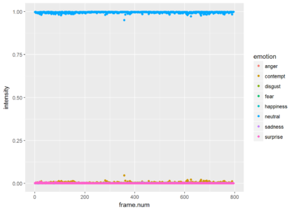
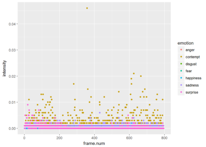
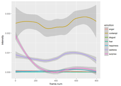
Since most of the frames show neutrality at a very high probability, the graph is not very informative. Just for the show, lets drop neutrality and focus on all other emotions. We can see that the is a small probability of some contempt during the video. The next plot shows only the points and the third plot shows only the smoothed version (without the points).
ggplot(res.for.gg %>% filter(emotion != "neutral"),
 aes(x = frame.num, y = intensity, color = emotion)) + geom_point()
ggplot(res.for.gg %>% filter(emotion != "neutral"),
 aes(x = frame.num, y = intensity, color = emotion)) + stat_smooth()

Conclusions

Though the Emotion API which used to analyze a complete video has been deprecated, the Face API can be used for this kind of video analysis, with the addition of splitting the video file to individual frames.

The possibilities with the face API are endless and can fit a variety of needs. Have fun playing around with it, and let me know if you found this tutorial helpful, or if you did something interesting with the API.

Shinydashboards from right to left (localizing a shinydashboard to Hebrew)

Post by Adi Sarid (Sarid Institute for Research Services LTD.)

Lately I’ve been working a lot with the shinydashboard library.
Like shiny, it allows any R programmer to harness the power of R and create professional looking interactive apps. The thing about shinydashboards is that it makes wonderfully looking dashboards.

What I’ve been doing with the dashboards is to create dedicated dashboards for my customers. Since most of my customers speak, read, and write in Hebrew I needed to fit that into my shinydashboard apps (i.e., fully localize the app). See an example for such a localized dashboard I made here.

Making a shinydashboard localized turned out to be simpler than I thought. 

Since the average R programmer doesn’t necessarily know and understand CSS, I thought I post my solution. This should fit any Hebrew or Arabic dashboard to work from right to left, including the sidebar and all other objects (though I only tested it in Hebrew).

If you want the short version:
(1) Download the following css file;
(2) Put it in a subfolder “/www” of your shinydashboard app;
(3) In your dashboardBody command (within the ui.R section of your shiny app) add the following code:
dashboardBody(
tags$head(
tags$link(rel = "stylesheet", type = "text/css", href = "bootstrap-rtl.css"
),...


Here are the few insights and steps which lead me to this solution:

Insight #1:
any shiny app (dashboard or otherwise) can be customized using CSS. That’s no secret. However, the adaptation to RTL isn’t that simple when you have so many objects, mobile responsiveness to worry about, etc.

Insight #2:
Shiny is based on the AdminLTE theme which is based on the bootstrap 3 theme. AdminLTE is a great theme, and even though it doesn’t officially support RTL, mmdsharifi, provided a solution in his github page. The same for bootstrap 3 which has an RTL customization by morteza (also on github).

Insight #3:
 What I did in order to make this work was to take the bootstrap-rtl.css from morteza, and then concatenate the AdminLTE-rtl.css file by mmdsharifi. Voilà! (simple, isn’t it?)

Here’s the resulting css file.

Thanks to 0xOri for suggesting and testing insight #3.


HebRew (using Hebrew in R)

Adi Sarid (Tel Aviv university and Sarid Research Institute LTD.)

July-2017

Background

A while back I participated in an R workshop, in the annual convention of the Israeli Association for Statistics. I had the pleasure of talking with Tal Galili and Jonathan Rosenblatt which indicated that a lot of Israeli R users run into difficulties with Hebrew with R. My firm opinion is that its best to keep everything in English, but sometimes you simply don’t have a choice. For example, I had to prepare a number of R shiny dashboards to Hebrew speaking clients, hence Hebrew was the way to go, in a kind of English-Hebrew “Mishmash” (mix). I happened to run into a lot of such difficulties in the past, so here are a few pointers to get you started when working in R with Hebrew. This post deals with Reading and writing files which contain Hebrew characters. Note, there is also a bit to talk about in the context of Shiny apps which contain Hebrew and using right-to-left in shiny apps, and using Hebrew variable names. Both work with some care, but I won’t cover them here. If you have any other questions you’d like to see answered, feel free to contact me [email protected].

Reading and writing files with Hebrew characters

R can read and write files in many formats. The common formats for small to medium data sets include the comma separated values (*.csv), and excel files (*.xlsx, *.xls). Each such read/write action is facilitated using some kind of “encoding”. Encoding, in simple terms, is a definition of a character set which help you operating system to interpret and represent the character as it should (לדוגמה, תווים בעברית). There are a number of relevant character sets (encodings) when Hebrew is concerned:
  • UTF-8
  • ISO 8859-8
  • Windows-1255
When you try to read files in which there are Hebrew characters, I usually recommend trying to read them in that order- UTF-8 is commonly used by a lot of applications, since it covers a lot of languages.

Using csv files with Hebrew characters

Here’s an example for something that can go wrong, and a possible solution. In this case I’ve prepared a csv file which encoded with UTF-8. When using R’s standard read.csv function, this is what happens:
sample.data <- read.csv("http://www.sarid-ins.co.il/files/utf_encoded_sample.csv")
sample.data
##    ן...... X......        X............
## 1 ׳¨׳•׳ ׳™      25             ׳—׳™׳₪׳”
## 2 ׳ž׳•׳˜׳™      77         ׳”׳¨׳¦׳œ׳™׳”
## 3   ׳“׳ ׳™      13 ׳×׳œ-׳׳‘׳™׳‘ ׳™׳₪׳•
## 4 ׳¨׳¢׳•׳×      30  ׳§׳¨׳™׳× ׳©׳ž׳•׳ ׳”
## 5   ׳“׳ ׳”      44        ׳‘׳™׳× ׳©׳׳Ÿ
Oh boy, that’s probably not what the file’s author had in mind. Let’s try to instruct read.csv to use a different encoding.
sample.data <- read.csv("http://www.sarid-ins.co.il/files/utf_encoded_sample.csv",
                        encoding = "UTF-8")
sample.data
##   X.U.FEFF.שם גיל      מגורים
## 1        רוני  25        חיפה
## 2        מוטי  77      הרצליה
## 3         דני  13 תל-אביב יפו
## 4        רעות  30  קרית שמונה
## 5         דנה  44     בית שאן
A bit better isn’t it? However, not perfect. We can read the Hebrew, but there is a weird thing in the header “X.U.FEFF”. A better way to read and write files (much more than just encoding aspects – it’s quicker reading large files) is using the readr package which is part of the tidyverse. On a side note, if you haven’t already, install.packages(tidyverse), it’s a must. It includes readr but a lot more goodies (read on). Now, for some tools you get with readr:
library(readr)
locale("he")
## <locale>
## Numbers:  123,456.78
## Formats:  %AD / %AT
## Timezone: UTC
## Encoding: UTF-8
## <date_names>
## Days:   יום ראשון (יום א׳), יום שני (יום ב׳), יום שלישי (יום ג׳), יום
##         רביעי (יום ד׳), יום חמישי (יום ה׳), יום שישי (יום ו׳), יום
##         שבת (שבת)
## Months: ינואר (ינו׳), פברואר (פבר׳), מרץ (מרץ), אפריל (אפר׳), מאי (מאי),
##         יוני (יוני), יולי (יולי), אוגוסט (אוג׳), ספטמבר (ספט׳),
##         אוקטובר (אוק׳), נובמבר (נוב׳), דצמבר (דצמ׳)
## AM/PM:  לפנה״צ/אחה״צ
guess_encoding("http://www.sarid-ins.co.il/files/utf_encoded_sample.csv")
## # A tibble: 2 × 2
##   encoding confidence
##      <chr>      <dbl>
## 1    UTF-8       1.00
## 2   KOI8-R       0.98
First we used locale() which knows the date format and default encoding for the language (UTF-8 in this case). On it’s own locale() does nothing than output the specs of the locale, but when used in conjuction with read_csv it tells read_csv everything it needs to know. Also note the use of guess_encoding which reads the first “few” lines of a file (10,000 is the default) which helps us, well… guess the encoding of a file. You can see that readr is pretty confident we need the UTF-8 here (and 98% confident we need a Korean encoding, but first option wins here…)
sample.data <- read_csv(file = "http://www.sarid-ins.co.il/files/utf_encoded_sample.csv",
                        locale = locale(date_names = "he", encoding = "UTF-8"))
## Parsed with column specification:
## cols(
##   שם = col_character(),
##   גיל = col_integer(),
##   מגורים = col_character()
## )
sample.data
## # A tibble: 5 × 3
##      שם   גיל      מגורים
##   <chr> <int>       <chr>
## 1  רוני    25        חיפה
## 2  מוטי    77      הרצליה
## 3   דני    13 תל-אביב יפו
## 4  רעות    30  קרית שמונה
## 5   דנה    44     בית שאן
Awesome isn’t it? Note that the resulting sample.data is a tibble and not a data.frame (read about tibbles). The package readr has tons of functions features to help us with reading (writing) and controlling the encoding, so I definitely recommend it. By the way, try using read_csv without setting the locale parameter and see what happens.

What about files saved by Excel?

Excel files are not the best choice for storing datasets, but the format is extremely common for obvious reasons.

CSV files which were saved by excel

In the past, I had run to a lot of difficulties trying to load CSV files which were saved by excel into R. Excel seems to save them in either “Windows-1255” or “ISO-8859-8”, instead of “UTF-8”. The default read by read_csv might yield something like “” instead of “שלום”. In other cases you might get a “multibyte error”. Just make sure you check the “Windows-1255” or “ISO-8859-8” encodings if the standard UTF-8 doesn’t work well (i.e., use read_csv(file, locale = locale(encoding = "ISO-8859-8"))).

Reading directly from excel

Also, if the original is in Excel, you might want to consider reading it directly from the excel file (skipping CSVs entirely). There are a number of packages for reading excel files and I recommend using readxl, specifically read_xlsx or read_xls will do the trick (depending on file format). You don’t even have to specify the encoding, if there are Hebrew characters they will be read as they should be.

Summary

For reading csv files with Hebrew characters, it’s very convenient to use readr. The package has a lot of utilities for language encoding and localization like guess_encoding and locale. If the original data is in excel, you might want to try skipping the csv and read the data directly from the excel format using the readxl package. Somtimes reading files envolves a lot of trial and error – but eventually it will work.

Don’t give up!