How to extract data from a PDF file with R


In this post, taken from the book R Data Mining by Andrea Cirillo, we’ll be looking at how to scrape PDF files using R. It’s a relatively straightforward way to look at text mining – but it can be challenging if you don’t know exactly what you’re doing.

Until January 15th, every single eBook and video by Packt is just $5! Start exploring some of Packt’s huge range of R titles here.

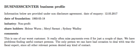
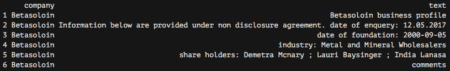
You may not be aware of this, but some organizations create something called a ‘customer card’ for every single customer they deal with. This is quite an informal document that contains some relevant information related to the customer, such as the industry and the date of foundation. Probably the most precious information contained within these cards is the comments they write down about the customers. Let me show you one of them:
My plan was the following—get the information from these cards and analyze it to discover whether some kind of common traits emerge.

As you may already know, at the moment this information is presented in an unstructured way; that is, we are dealing with unstructured data. Before trying to analyze this data, we will have to gather it in our analysis environment and give it some kind of structure.

Technically, what we are going to do here is called text mining, which generally refers to the activity of gaining knowledge from texts. The techniques we are going to employ are the following:

  • Sentiment analysis
  • Wordclouds
  • N-gram analysis
  • Network analysis

Getting a list of documents in a folder

First of all, we need to get a list of customer cards we were from the commercial department. I have stored all of them within the ‘data’ folder on my workspace. Let’s use list.files() to get them:
file_vector <- list.files(path = "data")
Nice! We can inspect this looking at the head of it. Using the following command:
file_vector %>% head()

[1] "banking.xls" "Betasoloin.pdf" "Burl Whirl.pdf" "BUSINESSCENTER.pdf"
 [5] "Buzzmaker.pdf" "BuzzSaw Publicity.pdf"
Uhm… not exactly what we need. I can see there are also .xls files. We can remove them using the grepl() function, which performs partial matches on strings, returning TRUE if the pattern required is found, or FALSE if not. We are going to set the following test here: give me TRUE if you find .pdf in the filename, and FALSE if not:
grepl(".pdf",file_list)

[1] FALSE TRUE TRUE TRUE TRUE TRUE TRUE TRUE TRUE FALSE TRUE TRUE TRUE TRUE TRUE TRUE TRUE
[18] TRUE TRUE TRUE TRUE TRUE TRUE TRUE TRUE TRUE TRUE TRUE TRUE TRUE TRUE TRUE TRUE TRUE
[35] TRUE TRUE TRUE TRUE TRUE TRUE TRUE TRUE TRUE TRUE TRUE TRUE TRUE TRUE TRUE TRUE TRUE
[52] TRUE TRUE TRUE TRUE FALSE TRUE TRUE TRUE TRUE TRUE TRUE TRUE TRUE TRUE TRUE TRUE TRUE
[69] TRUE TRUE TRUE TRUE TRUE TRUE TRUE TRUE TRUE TRUE TRUE TRUE TRUE TRUE TRUE TRUE TRUE
[86] TRUE TRUE TRUE TRUE TRUE TRUE TRUE TRUE TRUE TRUE TRUE TRUE TRUE TRUE TRUE TRUE TRUE
[103] TRUE TRUE TRUE TRUE TRUE TRUE TRUE TRUE TRUE TRUE TRUE TRUE TRUE TRUE FALSE FALSE TRUE
[120] TRUE
As you can see, the first match results in a FALSE since it is related to the .xls file we saw before. We can now filter our list of files by simply passing these matching results to the list itself. More precisely, we will slice our list, selecting only those records where our grepl() call returns TRUE:
pdf_list <- file_vector[grepl(".pdf",file_list)]
Did you understand [grepl(“.pdf”,file_list)] ? It is actually a way to access one or more indexes within a vector, which in our case are the indexes corresponding to “.pdf”, exactly the same as we printed out before. If you now look at the list, you will see that only PDF filenames are shown on it.

Reading PDF files into R via pdf_text()

R comes with a really useful that’s employed tasks related to PDFs. This is named pdftools, and beside the pdf_text function we are going to employ here, it also contains other relevant functions that are used to get different kinds of information related to the PDF file into R. For our purposes, it will be enough to get all of the textual information contained within each of the PDF files. First of all, let’s try this on a single document; we will try to scale it later on the whole set of documents. The only required argument to make pdf_text work is the path to the document. The object resulting from this application will be a character vector of length 1:
pdf_text("data/BUSINESSCENTER.pdf")

[1] "BUSINESSCENTER business profile\nInformation below are provided under non disclosure agreement. date of enquery: 12.05.2017\ndate of foundation: 1993-05-18\nindustry: Non-profit\nshare holders: Helene Wurm ; Meryl Savant ; Sydney Wadley\ncomments\nThis is one of our worst customer. It really often miss payments even if for just a couple of days. We have\nproblems finding useful contact persons. The only person we can have had occasion to deal with was the\nfiscal expert, since all other relevant person denied any kind of contact.\n                                                       1\n"
If you compare this with the original PDF document you can easily see that all of the information is available even if it is definitely not ready to be analyzed. What do you think is the next step needed to make our data more useful? We first need to split our string into lines in order to give our data a structure that is closer to the original one, that is, made of paragraphs. To split our string into separate records, we can use the strsplit() function, which is a base R function. It requires the string to be split and the token that decides where the string has to be split as arguments. If you now look at the string, you’ll notice that where we found the end of a line in the original document, for instance after the words business profile, we now find the \n token. This is commonly employed in text formats to mark the end of a line. We will therefore use this token as a split argument:
pdf_text("data/BUSINESSCENTER.pdf") %>% strsplit(split = "\n")

[[1]]
 [1] "BUSINESSCENTER business profile"
 [2] "Information below are provided under non disclosure agreement. date of enquery: 12.05.2017"
 [3] "date of foundation: 1993-05-18"
 [4] "industry: Non-profit"
 [5] "share holders: Helene Wurm ; Meryl Savant ; Sydney Wadley"
 [6] "comments"
 [7] "This is one of our worst customer. It really often miss payments even if for just a couple of days. We have"
 [8] "problems finding useful contact persons. The only person we can have had occasion to deal with was the"
 [9] "fiscal expert, since all other relevant person denied any kind of contact."
 [10] " 1"
strsplit() returns a list with an element for each element of the character vector passed as argument; within each list element, there is a vector with the split string. Isn’t that better? I definitely think it is. The last thing we need to do before actually doing text mining on our data is to apply those treatments to all of the PDF files and gather the results into a conveniently arranged data frame.

Iteratively extracting text from a set of documents with a for loop

What we want to do here is run trough the list of files and for filename found there, we run the pdf_text() function and then the strsplit() function to get an object similar to the one we have seen with our test. A convenient way to do this is by employing a ‘for’ loop. These structures basically do this to their content: Repeat this instruction n times and then stop. Let me show you a typical ‘for’ loop:
for (i in 1:3){
 print(i)
}
If we run this, we obtain the following:
[1] 1
 [1] 2
 [1] 3
This means that the loop runs three times and therefore repeats the instructions included within the brackets three times. What is the only thing that seems to change every time? It is the value of i. This variable, which is usually called counter, is basically what the loop employs to understand when to stop iterating. When the loop execution starts, the loop starts increasing the value of the counter, going from 1 to 3 in our example. The for loop repeats the instructions between the brackets for each element of the values of the vector following the in clause in the for command. At each step, the value of the variable before in (i in this case) takes one value of the sequence from the vector itself. The counter is also useful within the loop itself, and it is usually employed to iterate within an object in which some kind of manipulation is desired. Take, for instance, a vector defined like this:
vector <- c(1,2,3)
Imagine we want to increase the value of every element of the vector by 1. We can do this by employing a loop such as this:
for (i in 1:3){
 vector[i] <- vector[i]+1
}
If you look closely at the loop, you’ll realize that the instruction needs to access the element of the vector with an index equal to i and modify this value by 1. The counter here is useful because it will allow iteration on all vectors from 1 to 3. Be aware that this is actually not a best practice because loops tend to be quite computationally expensive, and they should be employed when no other valid alternative is available. For instance, we can obtain the same result here by working directly on the whole vector, as follows:
vector_increased <- vector +1
If you are interested in the topic of avoiding loops where they are not necessary, I can share with you some relevant material on this. For our purposes, we are going to apply loops to go through the pdf_list object, and apply the pdf_text function and subsequently the strsplit() function to each element of this list:
corpus_raw <- data.frame("company" = c(),"text" = c())

for (i in 1:length(pdf_list)){
print(i)
 pdf_text(paste("data/", pdf_list[i],sep = "")) %>% 
 strsplit("\n")-> document_text
data.frame("company" = gsub(x =pdf_list[i],pattern = ".pdf", replacement = ""), 
 "text" = document_text, stringsAsFactors = FALSE) -> document

colnames(document) <- c("company", "text")
corpus_raw <- rbind(corpus_raw,document) 
}
Let’s get closer to the loop: we first have a call to the pdf_text function, passing an element of pdf_list as an argument; it is defined as referencing the i position in the list. Once we have done this, we can move on to apply the strsplit() function to the resulting string. We define the document object, which contains two columns, in this way:
  • company, which stores the name of the PDF without the .pdf token; this is the name of the company
  • text, which stores the text resulting from the extraction
This document object is then appended to the corpus object, which we created previously, to store all of the text within the PDF. Let’s have a look a the resulting data frame:
corpus_raw %>% head()

This is a well-structured object, ready for some text mining. Nevertheless, if we look closely at our PDF customer cards, we can see that there are three different kinds of information and they should be handled differently:
  • Repeated information, such as the confidentiality disclosure on the second line and the date of enquiry (12.05.2017)
  • Structured attributes, for instance, date of foundation or industry
  • Strictly unstructured data, which is in the comments paragraph
We are going to address these three kinds of data differently, removing the first group of irrelevant information; we therefore have to split our data frame accordingly into two smaller data frames. To do so, we will leverage the grepl() function once again, looking for the following tokens:

  • 12.05.2017: This denotes the line showing the non-disclosure agreement and the date of inquiry.
  • business profile: This denotes the title of the document, containing the name of the company. We already have this information stored within the company column.
  • comments: This is the name of the last paragraph.
  • 1: This represents the number of the page and is always the same on every card.
We can apply the filter function to our corpus_raw object here as follows:
corpus_raw %>% 
filter(!grepl("12.05.2017",text)) %>% 
filter(!grepl("business profile",text)) %>% 
filter(!grepl("comments",text)) %>%
filter(!grepl("1",text)) -> corpus
Now that we have removed those useless things, we can actually split the data frame into two sub-data frames based on what is returned by the grepl function when searching for the following tokens, which point to the structured attributes we discussed previously:
  • date of foundation
  • industry
  • shareholders

We are going to create two different data frames here; one is called ‘information’ and the other is called ‘comments’:
corpus %>% 
filter(!grepl(c("date of foundation"),text)) %>% 
filter(!grepl(c( "industry"),text)) %>% 
filter(!grepl(c( "share holders"),text)) -> comments

corpus %>% 
filter(grepl(("date of foundation"),text)|grepl(( "industry"),text)|grepl(( "share holders"),text))-> information
As you can see, the two data treatments are nearly the opposite of each other, since the first looks for lines showing none of the three tokens while the other looks for records showing at least one of the tokens. Let’s inspect the results by employing the head function:
information %>% head()
comments %>% head()
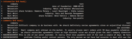
Great! We are nearly done. We are now going to start analyzing the comments data frame, which reports all comments from our colleagues. The very last step needed to make this data frame ready for subsequent analyzes is to tokenize it, which basically means separating it into different rows for all the words available within the text column. To do this, we are going to leverage the unnest_tokens function, which basically splits each line into words and produces a new row for each word, having taken care to repeat the corresponding value within the other columns of the original data frame. This function comes from the recent tidytext package by Julia Silge and Davide Robinson, which provides an organic framework of utilities for text mining tasks. It follows the tidyverse framework, which you should already know about if you are using the dplyr package. Let’s see how to apply the unnest_tokens function to our data:
comments %>% 
 unnest_tokens(word,text)-> comments_tidy
If we now look at the resulting data frame, we can see the following:

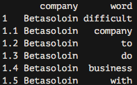
As you can see, we now have each word separated into a single record.

Thanks for reading! We hope you enjoyed this extract taken from R Data Mining.

Explore $5 R eBooks and videos from Packt until January 15th 2018.  

How to identify risky bank loans using C.50 decision trees

This tutorial has been taken from Machine Learning with R Second Edition   by Brett Lantz. Use the code  MLR250RB at the checkout to save 50% on the RRP.

Or pick up this title with 4 others for just $50 – get the R-Bloggers bundle.

The global financial crisis of 2007-2008 highlighted the importance of transparency and rigor in banking practices. As the availability of credit was limited, banks tightened their lending systems and turned to machine learning to more accurately identify risky loans. Decision trees are widely used in the banking industry due to their high accuracy and ability to formulate a statistical model in plain language. Since government organizations in many countries carefully monitor lending practices, executives must be able to explain why one applicant was rejected for a loan while the others were approved. This information is also useful for customers hoping to determine why their credit rating is unsatisfactory. It is likely that automated credit scoring models are employed to instantly approve credit applications on the telephone and web. In this tutorial, we will develop a simple credit approval model using C5.0 decision trees. We will also see how the results of the model can be tuned to minimize errors that result in a financial loss for the institution.

Step 1 – collecting data

The idea behind our credit model is to identify factors that are predictive of higher risk of default. Therefore, we need to obtain data on a large number of past bank loans and whether the loan went into default, as well as information on the applicant. Data with these characteristics is available in a dataset donated to the UCI Machine Learning Data Repository by Hans Hofmann of the University of Hamburg. The data set contains information on loans obtained from a credit agency in Germany.
The data set presented in this tutorial has been modified slightly from the original in order to eliminate some preprocessing steps. To follow along with the examples, download the credit.csv file from Packt’s website and save it to your R working directory. Simply click here and then click ‘code files’ beneath the cover image.
The credit data set includes 1,000 examples on loans, plus a set of numeric and nominal features indicating the characteristics of the loan and the loan applicant. A class variable indicates whether the loan went into default. Let’s see whether we can determine any patterns that predict this outcome.

Step 2 – exploring and preparing the data


As we did previously, we will import data using the read.csv() function. We will ignore the stringsAsFactors option and, therefore, use the default value of TRUE, as the majority of the features in the data are nominal:
> credit <- read.csv("credit.csv")

The first several lines of output from the str() function are as follows:
> str(credit)
'data.frame':1000 obs. of  17 variables:
 $ checking_balance : Factor w/ 4 levels "< 0 DM","> 200 DM",..
 $ months_loan_duration: int  6 48 12 ...
 $ credit_history      : Factor w/ 5 levels "critical","good",..
 $ purpose             : Factor w/ 6 levels "business","car",..
 $ amount              : int  1169 5951 2096 ...
We see the expected 1,000 observations and 17 features, which are a combination of factor and integer data types. Let’s take a look at the table() output for a couple of loan features that seem likely to predict a default. The applicant’s checking and savings account balance are recorded as categorical variables:
> table(credit$checking_balance)
    < 0 DM   > 200 DM 1 - 200 DM    unknown 
       274         63        269        394
> table(credit$savings_balance)
     < 100 DM > 1000 DM  100 - 500 DM 500 - 1000 DM   unknown 
          603        48           103            63       183
The checking and savings account balance may prove to be important predictors of loan default status. Note that since the loan data was obtained from Germany, the currency is recorded in Deutsche Marks (DM). Some of the loan’s features are numeric, such as its duration and the amount of credit requested:
> summary(credit$months_loan_duration)
   Min. 1st Qu.  Median    Mean 3rd Qu.    Max. 
    4.0    12.0    18.0    20.9    24.0    72.0 
> summary(credit$amount)
   Min. 1st Qu.  Median    Mean 3rd Qu.    Max. 
    250    1366    2320    3271    3972   18420
The loan amounts ranged from 250 DM to 18,420 DM across terms of 4 to 72 months with a median duration of 18 months and an amount of 2,320 DM. The default vector indicates whether the loan applicant was unable to meet the agreed payment terms and went into default. A total of 30 percent of the loans in this dataset went into default:
> table(credit$default)
 no yes 
700 300
A high rate of default is undesirable for a bank, because it means that the bank is unlikely to fully recover its investment. If we are successful, our model will identify applicants that are at high risk to default, allowing the bank to refuse credit requests.

Data preparation: Creating random training and test data sets

In this example, we’lll split our data into two portions: a training dataset to build the decision tree and a test dataset to evaluate the performance of the model on new data. We will use 90 percent of the data for training and 10 percent for testing, which will provide us with 100 records to simulate new applicants. We’ll use a random sample of the credit data for training. A random sample is simply a process that selects a subset of records at random. In R, the sample() function is used to perform random sampling. However, before putting it in action, a common practice is to set a seed value, which causes the randomization process to follow a sequence that can be replicated later on if desired. It may seem that this defeats the purpose of generating random numbers, but there is a good reason for doing it this way. Providing a seed value via the set.seed() function ensures that if the analysis is repeated in the future, an identical result is obtained. The following commands use the sample() function to select 900 values at random out of the sequence of integers from 1 to 1000. Note that the set.seed() function uses the arbitrary value 123. Omitting this seed will cause your training and testing split to differ from those shown in the remainder of this tutorial:
> set.seed(123)
> train_sample <- sample(1000, 900)
As expected, the resulting train_sample object is a vector of 900 random integers:
> str(train_sample)
 int [1:900] 288 788 409 881 937 46 525 887 548 453 ... 
By using this vector to select rows from the credit data, we can split it into the 90 percent training and 10 percent test datasets we desired. Recall that the dash operator used in the selection of the test records tells R to select records that are not in the specified rows; in other words, the test data includes only the rows that are not in the training sample.
> credit_train <- credit[train_sample, ]
> credit_test  <- credit[-train_sample, ]
If all went well, we should have about 30 percent of defaulted loans in each of the datasets:
> prop.table(table(credit_train$default))
       no       yes 
0.7033333 0.2966667 

> prop.table(table(credit_test$default))
  no  yes 
0.67 0.33
This appears to be a fairly even split, so we can now build our decision tree. Tip: If your results do not match exactly, ensure that you ran the command
set.seed(123)
immediately prior to creating the
train_sample
vector.

Step 3: Training a model on the data

We will use the C5.0 algorithm in the C50 package to train our decision tree model. If you have not done so already, install the package with install.packages(“C50”) and load it to your R session, using library(C50). The following syntax box lists some of the most commonly used commands to build decision trees. Compared to the machine learning approaches we used previously, the C5.0 algorithm offers many more ways to tailor the model to a particular learning problem, but more options are available. Once the C50package has been loaded, the ?C5.0Control command displays the help page for more details on how to finely-tune the algorithm.

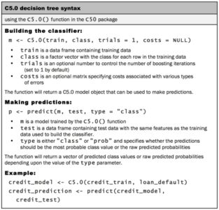
For the first iteration of our credit approval model, we’ll use the default C5.0 configuration, as shown in the following code. The 17th column in credit_train is the default class variable, so we need to exclude it from the training data frame, but supply it as the target factor vector for classification:
> credit_model <- C5.0(credit_train[-17], credit_train$default)
The credit_model object now contains a C5.0 decision tree. We can see some basic data about the tree by typing its name:
> credit_model

Call:
C5.0.default(x = credit_train[-17], y = credit_train$default)

Classification Tree
Number of samples: 900 
Number of predictors: 16 

Tree size: 57 

Non-standard options: attempt to group attributes
The preceding text shows some simple facts about the tree, including the function call that generated it, the number of features (labeled predictors), and examples (labeled samples) used to grow the tree. Also listed is the tree size of 57, which indicates that the tree is 57 decisions deep—quite a bit larger than the example trees we’ve considered so far! To see the tree’s decisions, we can call the summary() function on the model:
> summary(credit_model)
This results in the following output:

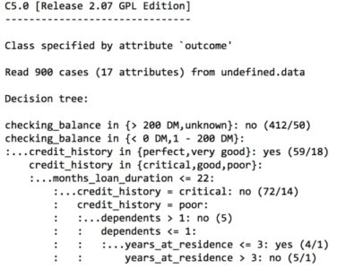
The preceding output shows some of the first branches in the decision tree. The first three lines could be represented in plain language as:

If the checking account balance is unknown or greater than 200 DM, then classify as “not likely to default.” Otherwise, if the checking account balance is less than zero DM or between one and 200 DM. And the credit history is perfect or very good, then classify as “likely to default.”

The numbers in parentheses indicate the number of examples meeting the criteria for that decision, and the number incorrectly classified by the decision. For instance, on the first line, 412/50 indicates that of the 412 examples reaching the decision, 50 were incorrectly classified as not likely to default. In other words, 50 applicants actually defaulted, in spite of the model’s prediction to the contrary. Tip: Sometimes a tree results in decisions that make little logical sense. For example, why would an applicant whose credit history is very good be likely to default, while those whose checking balance is unknown are not likely to default? Contradictory rules like this occur sometimes. They might reflect a real pattern in the data, or they may be a statistical anomaly. In either case, it is important to investigate such strange decisions to see whether the tree’s logic makes sense for business use.
After the tree, the summary(credit_model) output displays a confusion matrix, which is a cross-tabulation that indicates the model’s incorrectly classified records in the training data:
Evaluation on training data (900 cases):

      Decision Tree   
    ----------------  
    Size      Errors  
      56  133(14.8%)   <<

     (a)   (b)    <-classified as
    ----  ----
     598    35    (a): class no
      98   169    (b): class yes
The Errors output notes that the model correctly classified all but 133 of the 900 training instances for an error rate of 14.8 percent. A total of 35 actual no values were incorrectly classified as yes (false positives), while 98 yes values were misclassified as no (false negatives). Decision trees are known for having a tendency to overfit the model to the training data. For this reason, the error rate reported on training data may be overly optimistic, and it is especially important to evaluate decision trees on a test data set.

Step 4: Evaluating model performance

To apply our decision tree to the test dataset, we use the predict() function, as shown in the following line of code:
> credit_pred <- predict(credit_model, credit_test)
This creates a vector of predicted class values, which we can compare to the actual class values using the CrossTable() function in the gmodels package. Setting the prop.c and prop.r parameters to FALSE removes the column and row percentages from the table. The remaining percentage (prop.t) indicates the proportion of records in the cell out of the total number of records:
> library(gmodels)
> CrossTable(credit_test$default, credit_pred,
             prop.chisq = FALSE, prop.c = FALSE, prop.r = FALSE,
             dnn = c('actual default', 'predicted default'))
This results in the following table:


Out of the 100 test loan application records, our model correctly predicted that 59 did not default and 14 did default, resulting in an accuracy of 73 percent and an error rate of 27 percent. This is somewhat worse than its performance on the training data, but not unexpected, given that a model’s performance is often worse on unseen data. Also note that the model only correctly predicted 14 of the 33 actual loan defaults in the test data, or 42 percent. Unfortunately, this type of error is a potentially very costly mistake, as the bank loses money on each default. Let’s see if we can improve the result with a bit more effort.

Step 5: Improving model performance

Our model’s error rate is likely to be too high to deploy it in a real-time credit scoring application. In fact, if the model had predicted “no default” for every test case, it would have been correct 67 percent of the time—a result not much worse than our model’s, but requiring much less effort! Predicting loan defaults from 900 examples seems to be a challenging problem. Making matters even worse, our model performed especially poorly at identifying applicants who do default on their loans. Luckily, there are a couple of simple ways to adjust the C5.0 algorithm that may help to improve the performance of the model, both overall and for the more costly type of mistakes.

Boosting the accuracy of decision trees

One way the C5.0 algorithm improved upon the C4.5 algorithm was through the addition of adaptive boosting. This is a process in which many decision trees are built and the trees vote on the best class for each example. Boosting is essentially rooted in the notion that by combining a number of weak performing learners, you can create a team that is much stronger than any of the learners alone. Each of the models has a unique set of strengths and weaknesses and they may be better or worse in solving certain problems. Using a combination of several learners with complementary strengths and weaknesses can therefore dramatically improve the accuracy of a classifier. The C5.0() function makes it easy to add boosting to our C5.0 decision tree. We simply need to add an additional trials parameter indicating the number of separate decision trees to use in the boosted team. The trials parameter sets an upper limit; the algorithm will stop adding trees if it recognizes that additional trials do not seem to be improving the accuracy. We’ll start with 10 trials, a number that has become the de facto standard, as research suggests that this reduces error rates on test data by about 25%:
> credit_boost10 <- C5.0(credit_train[-17], credit_train$default,
                         trials = 10)
While examining the resulting model, we can see that some additional lines have been added, indicating the changes:
> credit_boost10
Number of boosting iterations: 10 
Average tree size: 47.5
Across the 10 iterations, our tree size shrunk. If you would like, you can see all 10 trees by typing summary(credit_boost10) at the command prompt. It also lists the model’s performance on the training data:
> summary(credit_boost10)

     (a)   (b)    <-classified as
    ----  ----
     629     4    (a): class no
      30   237    (b): class yes
The classifier made 34 mistakes on 900 training examples for an error rate of 3.8 percent. This is quite an improvement over the 13.9 percent training error rate we noted before adding boosting! However, it remains to be seen whether we see a similar improvement on the test data. Let’s take a look:
> credit_boost_pred10 <- predict(credit_boost10, credit_test)
> CrossTable(credit_test$default, credit_boost_pred10,
             prop.chisq = FALSE, prop.c = FALSE, prop.r = FALSE,
             dnn = c('actual default', 'predicted default'))
The resulting table is as follows:


Here, we reduced the total error rate from 27 percent prior to boosting down to 18 percent in the boosted model. It does not seem like a large gain, but it is in fact larger than the 25 percent reduction we expected. On the other hand, the model is still not doing well at predicting defaults, predicting only 20/33 = 61%correctly. The lack of an even greater improvement may be a function of our relatively small training data set, or it may just be a very difficult problem to solve.

This said, if boosting can be added this easily, why not apply it by default to every decision tree? The reason is twofold. First, if building a decision tree once takes a great deal of computation time, building many trees may be computationally impractical. Secondly, if the training data is very noisy, then boosting might not result in an improvement at all. Still, if greater accuracy is needed, it’s worth giving it a try.

Making mistakes more costlier than others

Giving a loan out to an applicant who is likely to default can be an expensive mistake. One solution to reduce the number of false negatives may be to reject a larger number of borderline applicants, under the assumption that the interest the bank would earn from a risky loan is far outweighed by the massive loss it would incur if the money is not paid back at all. The C5.0 algorithm allows us to assign a penalty to different types of errors, in order to discourage a tree from making more costly mistakes. The penalties are designated in a cost matrix, which specifies how much costlier each error is, relative to any other prediction. To begin constructing the cost matrix, we need to start by specifying the dimensions. Since the predicted and actual values can both take two values, yes or no, we need to describe a 2 x 2 matrix, using a list of two vectors, each with two values. At the same time, we’ll also name the matrix dimensions to avoid confusion later on:
> matrix_dimensions <- list(c("no", "yes"), c("no", "yes"))
> names(matrix_dimensions) <- c("predicted", "actual")
Examining the new object shows that our dimensions have been set up correctly:
> matrix_dimensions
$predicted
[1] "no"  "yes"

$actual
[1] "no"  "yes"
Next, we need to assign the penalty for the various types of errors by supplying four values to fill the matrix. Since R fills a matrix by filling columns one by one from top to bottom, we need to supply the values in a specific order:

  • Predicted no, actual no
  • Predicted yes, actual no
  • Predicted no, actual yes
  • Predicted yes, actual yes
Suppose we believe that a loan default costs the bank four times as much as a missed opportunity. Our penalty values could then be defined as:
> error_cost <- matrix(c(0, 1, 4, 0), nrow = 2,
    dimnames = matrix_dimensions)
This creates the following matrix:
> error_cost
         actual
predicted no yes
      no   0   4
      yes  1   0
As defined by this matrix, there is no cost assigned when the algorithm classifies a no or yes correctly, but a false negative has a cost of 4 versus a false positive’s cost of 1. To see how this impacts classification, let’s apply it to our decision tree using the costs parameter of the C5.0() function. We’ll otherwise use the same steps as we did earlier:
> credit_cost <- C5.0(credit_train[-17], credit_train$default,
                            costs = error_cost)
> credit_cost_pred <- predict(credit_cost, credit_test)
> CrossTable(credit_test$default, credit_cost_pred,
             prop.chisq = FALSE, prop.c = FALSE, prop.r = FALSE,
             dnn = c('actual default', 'predicted default'))
This produces the following confusion matrix:


Compared to our boosted model, this version makes more mistakes overall: 37 percent error here versus 18 percent in the boosted case. However, the types of mistakes are very different. Where the previous models incorrectly classified only 42 and 61 percent of defaults correctly, in this model, 79 percent of the actual defaults were predicted to be non-defaults. This trade resulting in a reduction of false negatives at the expense of increasing false positives may be acceptable if our cost estimates were accurate.

This tutorial has been taken from Machine Learning with R Second Edition   by Brett Lantz. Use the code  MLR250RB at the checkout to save 50% on the RRP.