This logging of digital communication is on the one hand interesting for researchers seeking to investigate interpersonal communication, social relationships, and linguistics, and can on the other hand also be interesting for individuals seeking to learn more about their own chatting behavior (or their social relationships).
The WhatsR R-package enables users to transform exported WhatsApp chat logs into a usable data frame object with one row per sent message and multiple variables of interest. In this blog post, I will demonstrate how the package can be used to process and visualize chat log files.
Installing the Package
The package can either be installed via CRAN or via GitHub for the most up-to-date version. I recommend to install the GitHub version for the most recent features and bugfixes.
# from CRAN
# install.packages("WhatsR")

# from GitHub
devtools::install_github("gesiscss/WhatsR")
The package also needs to be attached before it can be used. For creating nicer plots, I recommend to also install and attach the patchwork package.# installing patchwork package
install.packages("patchwork")
# attaching packages
library(WhatsR)
library(patchwork)
Obtaining a Chat LogYou can export one of your own chat logs from your phone to your email address as explained in this tutorial. If you do this, I recommend to use the “without media” export option as this allows you to export more messages.
If you don’t want to use one of your own chat logs, you can create an artificial chat log with the same structure as a real one but with made up text using the WhatsR package!
## creating chat log for demonstration purposes

# setting seed for reproducibility
set.seed(1234)

# simulating chat log
# (and saving it automatically as a .txt file in the working directory)
create_chatlog(n_messages = 20000,
               n_chatters = 5,
               n_emoji = 5000,
               n_diff_emoji = 50,
               n_links = 999,
               n_locations = 500,
               n_smilies = 2500,
               n_diff_smilies = 10,
               n_media = 999,
               n_sdp = 300,
               startdate = "01.01.2019",
               enddate = "31.12.2023",
               language = "english",
               time_format = "24h",
               os = "android",
               path = getwd(),
               chatname = "Simulated_WhatsR_chatlog")
Parsing Chat Log File
Once you have a chat log on your device, you can use the WhatsR package to import the chat log and parse it into a usable data frame structure.
data <- parse_chat("Simulated_WhatsR_chatlog.txt", verbose = TRUE)
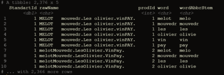
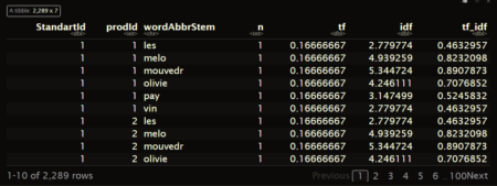
Checking the parsed Chat LogYou should now have a data frame object with one row per sent message and 19 variables with information extracted from the individual messages. For a detailed overview what each column contains and how it is computed, you can check the related open source publication for the package. We also add a tabular overview here.
## Checking the chat log
dim(data)
colnames(data)
|
Column Name |
Description |
|---|---|
|
DateTime |
Timestamp for date and time the message was sent. Formatted as yyyy-mm-dd hh:mm:ss |
|
Sender |
Name of the sender of the message as saved in the contact list of the exporting phone or telephone number. Messages inserted by WhatsApp into the chat are coded with “WhatsApp System Message” |
|
Message |
Text of user-generated messages with all information contained in the exported chat log |
|
Flat |
Simplified version of the message with emojis, numbers, punctuation, and URLs removed. Better suited for some text mining or machine learning tasks |
|
TokVec |
Tokenized version of the Flat column. Instead of one text string, each cell contains a list of individual words. Better suited for some text mining or machine learning tasks |
|
URL |
A list of all URLs or domains contained in the message body |
|
Media |
A list of all media attachment filenames contained in the message body |
|
Location |
A list of all shared location URLs or indicators in the message body, or indicators for shared live locations |
|
Emoji |
A list of all emoji glyphs contained in the message body |
|
EmojiDescriptions |
A list of all emojis as textual representations contained in the message body |
|
Smilies |
A list of all smileys contained in the message body |
|
SystemMessage |
Messages that are inserted by WhatsApp into the conversation and not generated by users |
|
TokCount |
Amount of user-generated tokens per message |
|
TimeOrder |
Order of messages as per the timestamps on the exporting phone |
|
DisplayOrder |
Order of messages as they appear in the exported chat log |
Now, you can have a first look at the overall statistics of the chat log. You can check the number of messages, sent tokens, number of chat participants, date of first message, date of last message, the timespan of the chat, and the number of emoji, smilies, links, media files, as well as locations in the chat log.
# Summary statistics
summarize_chat(data, exclude_sm = TRUE)
We can also check the distribution of the number of tokens per message and a set of summary statistics for each individual chat participant.
# Summary statistics
summarize_tokens_per_person(data, exclude_sm = TRUE)
Visualizing Chat Logs
The chat characteristics can now be visualized using the custom functions from the WhatsR package. These functions are basically wrappers to ggplot2 with some options for customizing the plots. Most plots have multiple ways of visualizing the data. For the visualizations, we can exclude the WhatsApp System Messages using ‘exclude_sm= TRUE’. Lets try it out:
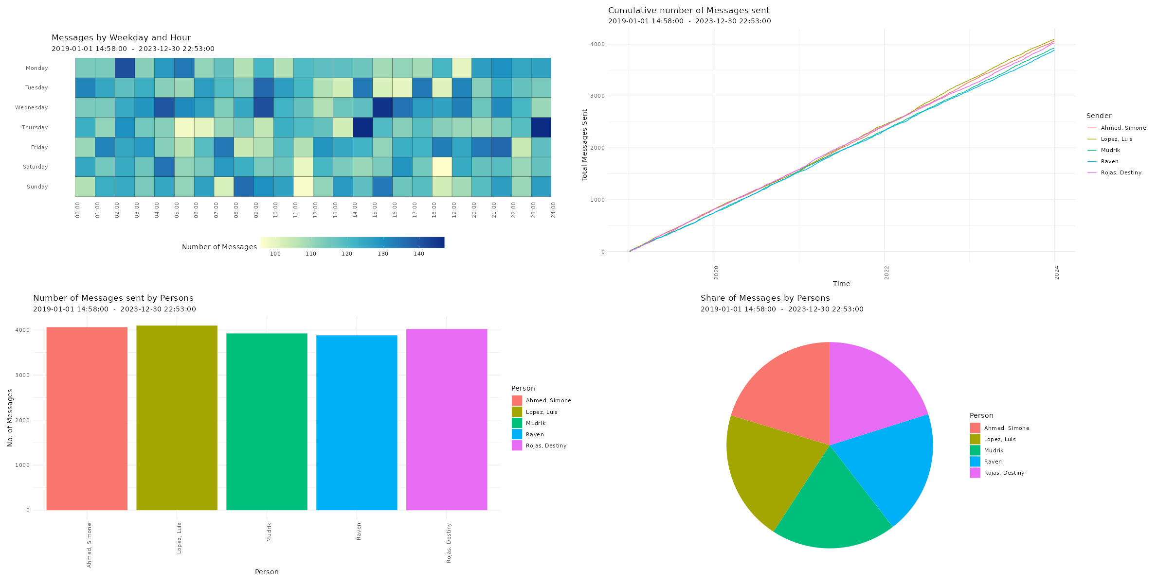
Amount of sent messages
# Plotting amount of messages
p1 <- plot_messages(data, plot = "bar", exclude_sm = TRUE)
p2 <- plot_messages(data, plot = "cumsum", exclude_sm = TRUE)
p3 <- plot_messages(data, plot = "heatmap", exclude_sm = TRUE)
p4 <- plot_messages(data, plot = "pie", exclude_sm = TRUE)

# Printing plots with patchwork package
(free(p3) | free(p2)) / (free(p1) | free(p4))
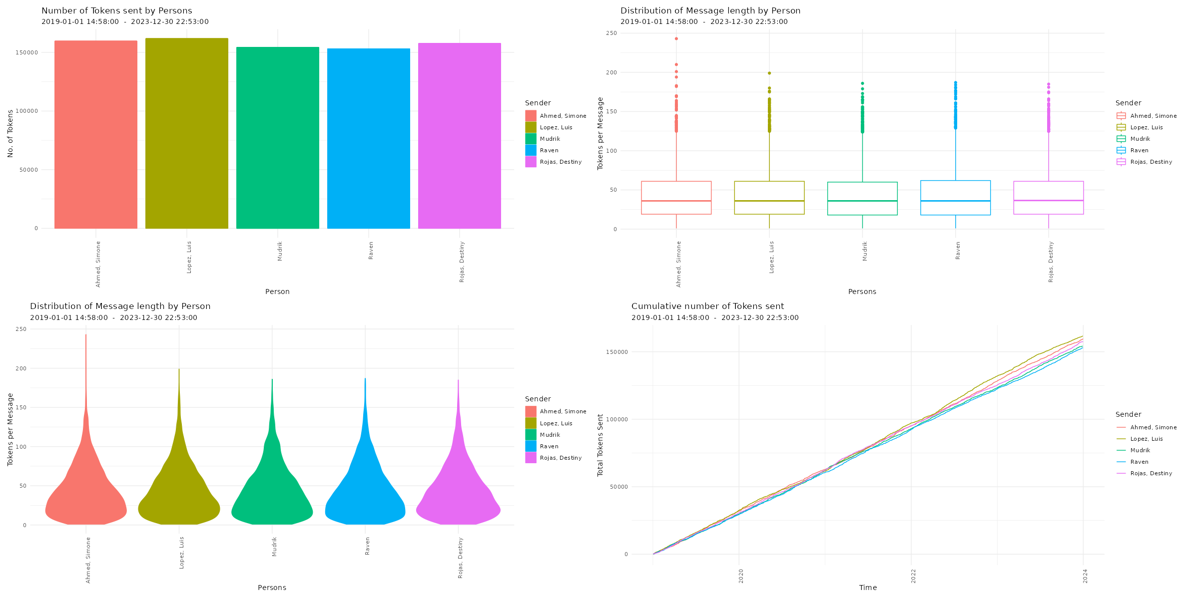
Amount of sent tokens
# Plotting amount of messages
p5 <- plot_tokens(data, plot = "bar", exclude_sm = TRUE)
p6 <- plot_tokens(data, plot = "box", exclude_sm = TRUE)
p7 <- plot_tokens(data, plot = "violin", exclude_sm = TRUE)
p8 <- plot_tokens(data, plot = "cumsum", exclude_sm = TRUE)

# Printing plots with patchwork package
(free(p5) | free(p6)) / (free(p7) | free(p8))
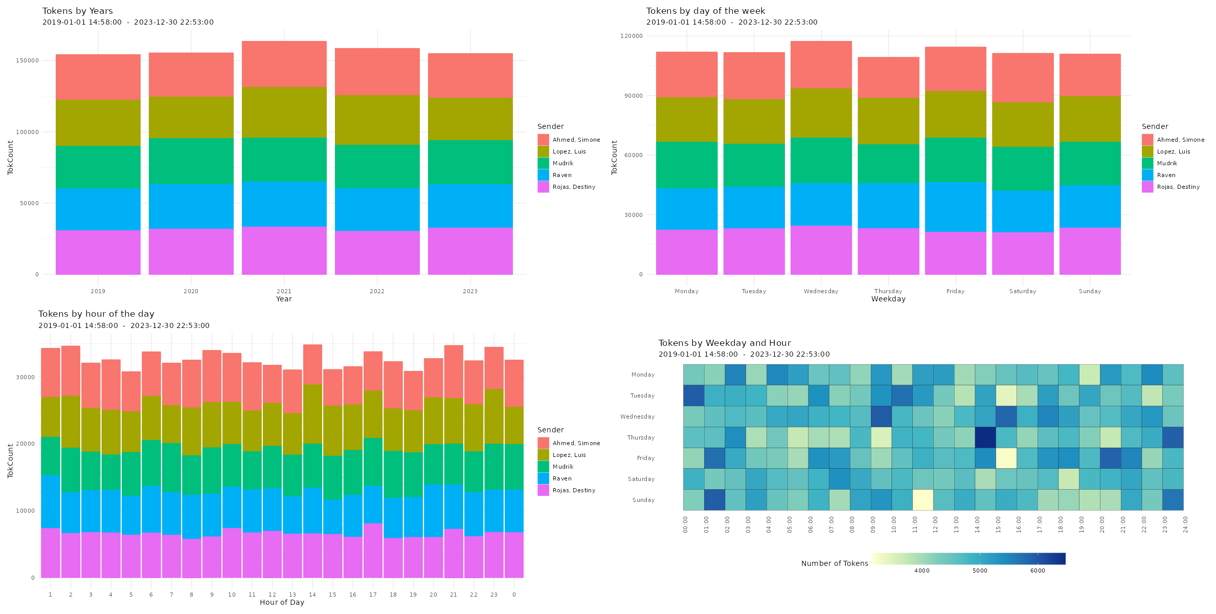
Amount of sent tokens over time
# Plotting amount of tokens over time
p9 <- plot_tokens_over_time(data,
                            plot = "year",
                            exclude_sm = TRUE)

p10 <- plot_tokens_over_time(data,
                             plot = "day",
                             exclude_sm = TRUE)

p11 <- plot_tokens_over_time(data,
                             plot = "hour",
                             exclude_sm = TRUE)

p12 <- plot_tokens_over_time(data,
                             plot = "heatmap",
                             exclude_sm = TRUE)

p13 <- plot_tokens_over_time(data,
                             plot = "alltime",
                             exclude_sm = TRUE)

# Printing plots with patchwork package
(free(p9) | free(p10)) / (free(p11) | free(p12))
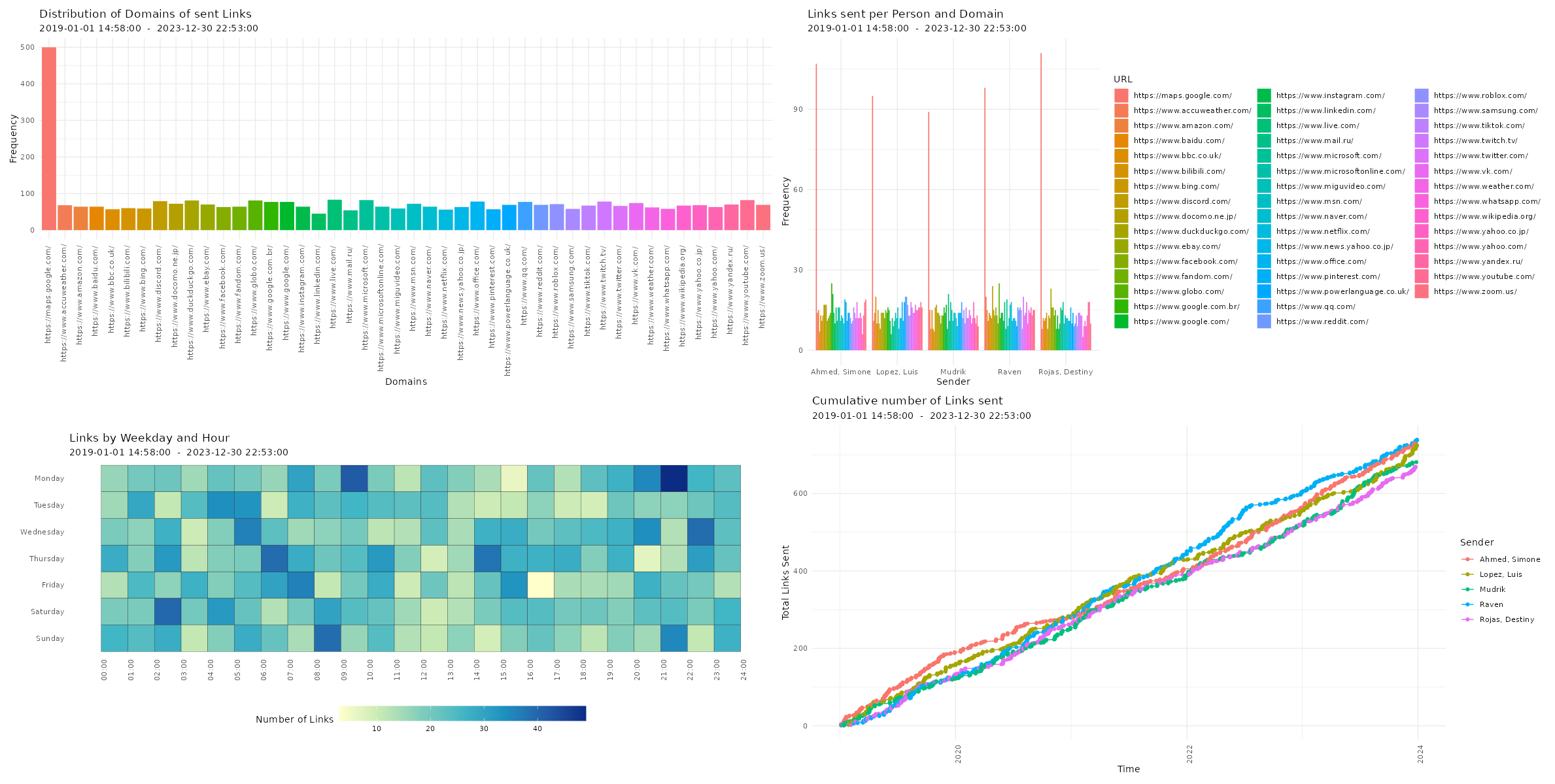
Amount of sent links
# Plotting amount of links
p14 <- plot_links(data, plot = "bar", exclude_sm = TRUE)
p15 <- plot_links(data, plot = "splitbar", exclude_sm = TRUE)
p16 <- plot_links(data, plot = "heatmap", exclude_sm = TRUE)
p17 <- plot_links(data, plot = "cumsum", exclude_sm = TRUE)

# Printing plots with patchwork package
(free(p14) | free(p15)) / (free(p16) | free(p17))
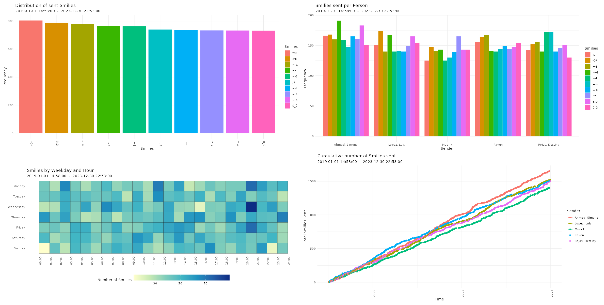
Amount of sent smilies
# Plotting amount of smilies
p18 <- plot_smilies(data, plot = "bar", exclude_sm = TRUE)
p19 <- plot_smilies(data, plot = "splitbar", exclude_sm = TRUE)
p20 <- plot_smilies(data, plot = "heatmap", exclude_sm = TRUE)
p21 <- plot_smilies(data, plot = "cumsum", exclude_sm = TRUE)

# Printing plots with patchwork package
(free(p18) | free(p19)) / (free(p20) | free(p21))
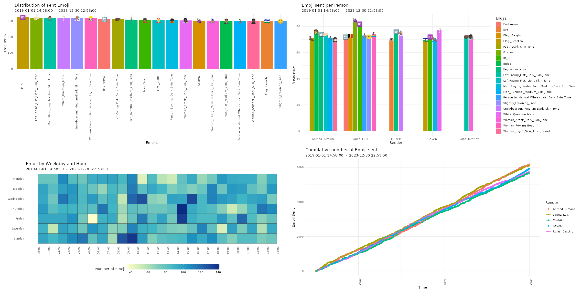
Amount of sent emoji
# Plotting amount of messages
p22 <- plot_emoji(data,
 plot = "bar",
 min_occur = 300,
 exclude_sm = TRUE,
 emoji_size=5)

p23 <- plot_emoji(data,
 plot = "splitbar",
 min_occur = 70,
 exclude_sm = TRUE,
 emoji_size=5)

p24 <- plot_emoji(data,
 plot = "heatmap",
 min_occur = 300,
 exclude_sm = TRUE)

p25 <- plot_emoji(data,
 plot = "cumsum",
 min_occur = 300,
 exclude_sm = TRUE)

# Printing plots with patchwork package
(free(p22) | free(p23)) / (free(p24) | free(p25))
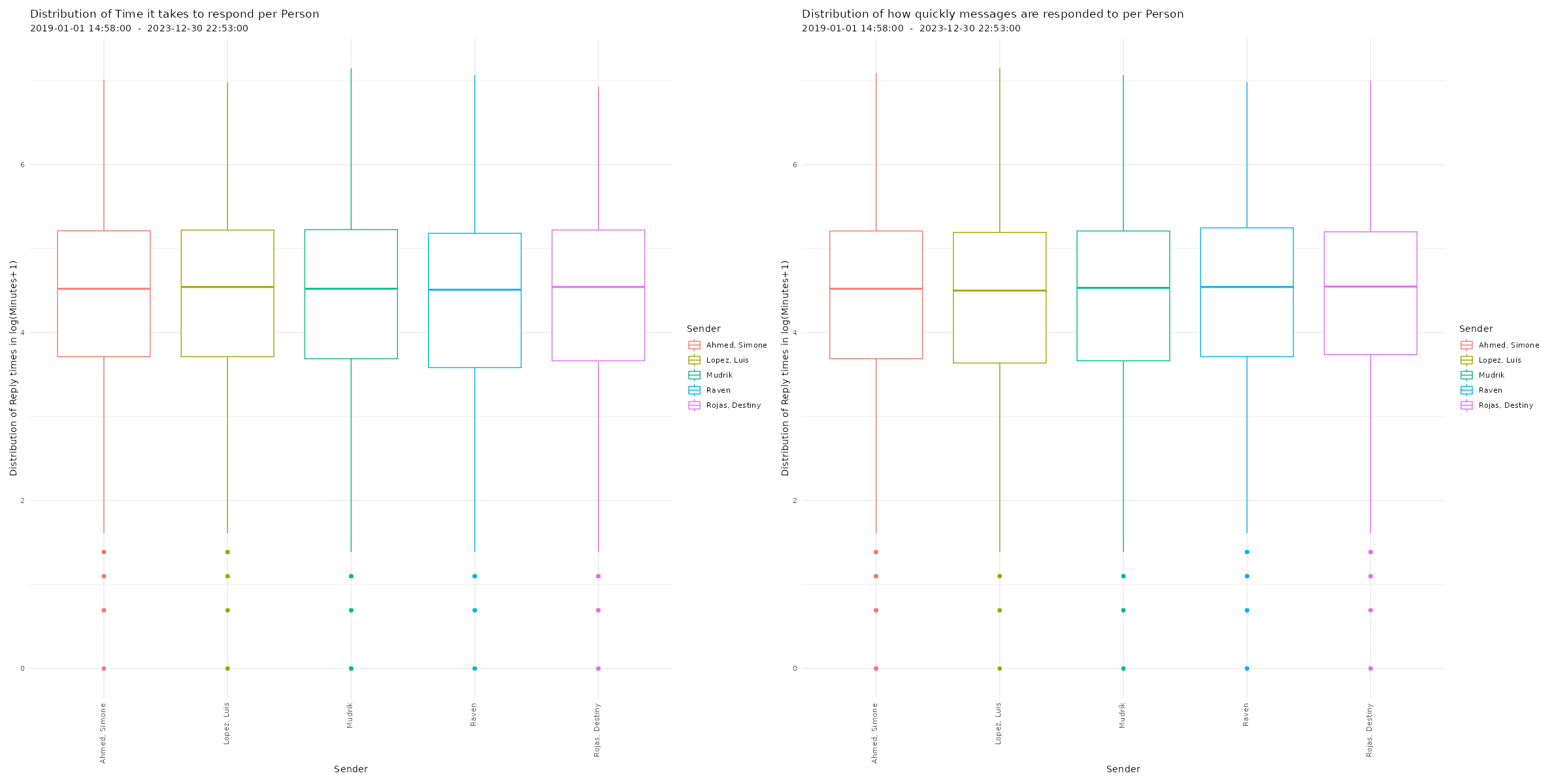
Distribution of reaction times
# Plotting distribution of reaction times
p26 <- plot_replytimes(data,
                       type = "replytime",
                       exclude_sm = TRUE)
p27 <- plot_replytimes(data,
                       type = "reactiontime",
                       exclude_sm = TRUE)

# Printing plots with patchwork package
free(p26) | free(p27)
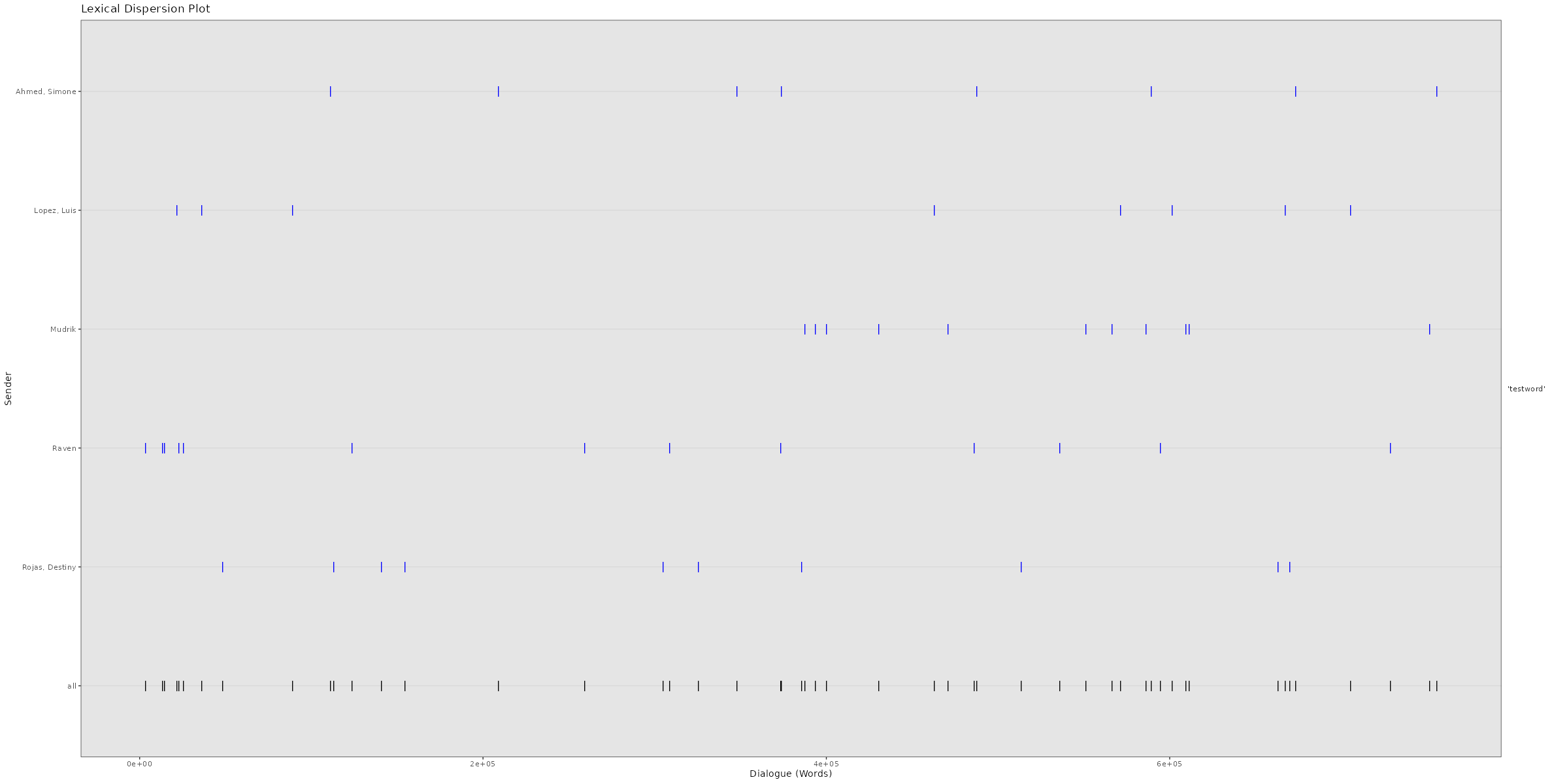
Lexical Dispersion
A lexical dispersion plot is a visualization of where specific words occur within a text corpus. Because the simulated chat log in this example is using lorem ipsum text where all words occur similarly often, we add the string “testword” to a random subsample of messages. For visualizing real chat logs, this would of course not be necessary.
# Adding "testword" to random subset of messages for demonstration         # purposes
set.seed(12345)
word_additions <- sample(dim(data)[1],50)
data$TokVec[word_additions]
sapply(data$TokVec[word_additions],function(x){c(x,"testword")})
data$Flat[word_additions] <- sapply(data$Flat[word_additions],
  function(x){x <- paste(x,"testword");return(x)})
Now you can create the lexical dispersion plot:# Plotting lexical dispersion plot
plot_lexical_dispersion(data,
keywords = c("testword"),
exclude_sm = TRUE)
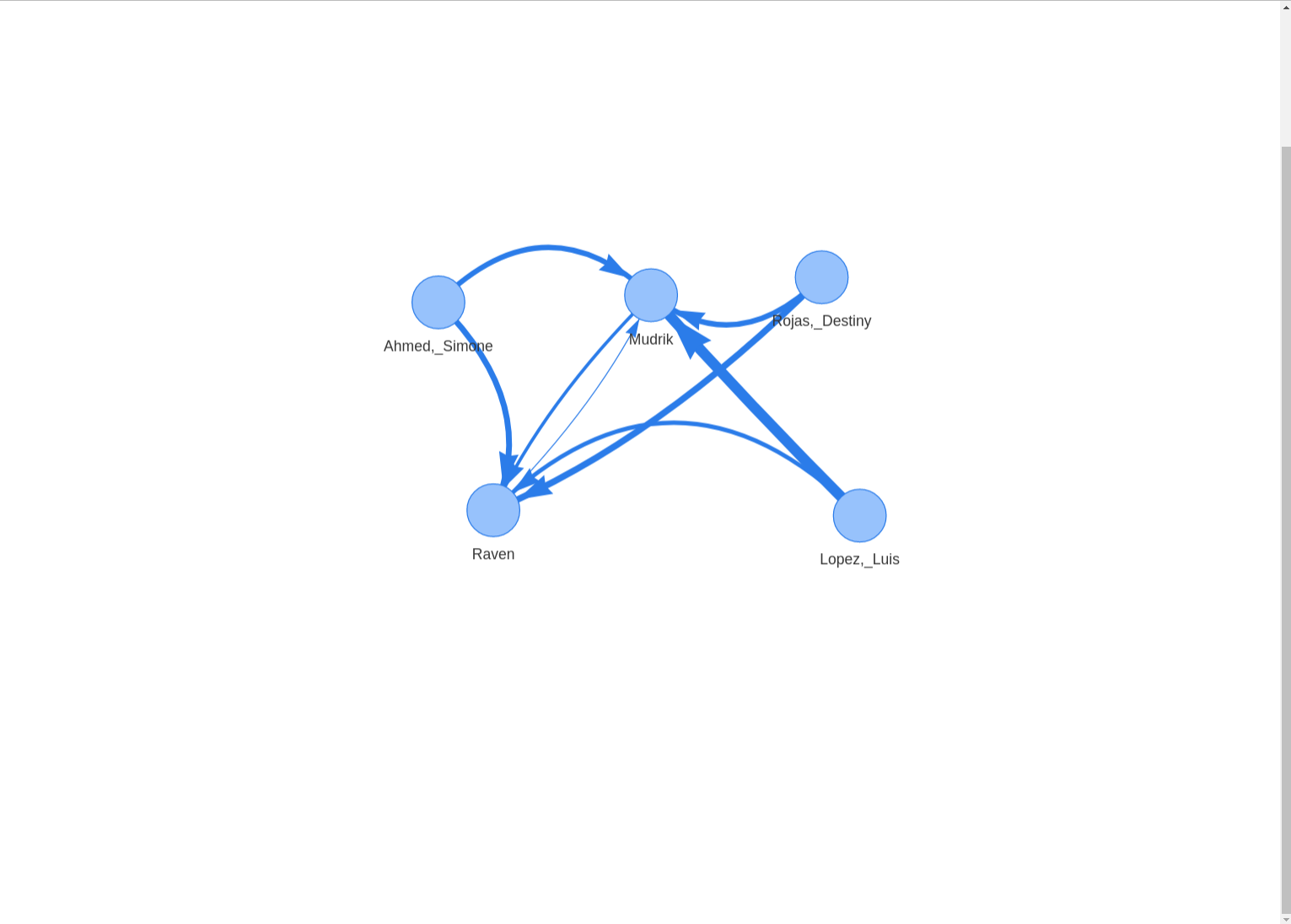
Response Networks
# Plotting response network
plot_network(data,
             edgetype = "n",
             collapse_sessions = TRUE,
             exclude_sm = TRUE)
Issues and long-term availability.
Unfortunately, WhatsApp chat logs are a moving target when it comes to plotting and visualization. The structure of exported WhatsApp chat logs keeps changing from time to time. On top of that, the structure of chat logs is different for chats exported from different operating systems (Android & iOS) and for different time (am/pm vs. 24h format) and language (e.g. English & German) settings on the exporting phone. When the structure changes, the WhatsR package can be limited in its functionality or become completely dysfunctional until it is updated and tested. Should you encounter any issues, all reports on the GitHub issues page are welcome. Should you want to contribute to improving on or maintaining the package, pull requests and collaborations are also welcome!