Azure Machine Learning For R Practitioners With The R SDK

[This article was first published on the Azure Medium channel, and kindly contributed to R-bloggers]. (You can report issue about the content on this page here)

As probably you already know, Microsoft provided its Azure Machine Learning SDK for Python to build and run machine learning workflows, helping organizations to use massive data sets and bring all the benefits of the Azure cloud to machine learning.

Although Microsoft initially invested in R as the Advanced Analytics preferred language introducing the SQL Server R server and R services in the 2016 version, they abruptly shifted their attention to Python, investing exclusively on it. This basically happened for the following reasons:

Python’s simple syntax and readability make the language accessible to non-programmers
The most popular machine learning and deep learning open source libraries (such as Pandas, scikit-learn, TensorFlow, PyTorch, etc.) are deeply used by the Python community
Python is a better choice for productionalization: it’s relatively very fast; it implements OOPs concepts in a better way; it is scalable (Hadoop/Spark); it has better functionality to interact with other systems; etc.

Azure ML Python SDK Main Key Points

One of the most valuable aspects of the Python SDK is its ease to use and flexibility. You can simply use just few classes, injecting them into your existing code or simply referring to your script files into method calls, in order to accomplish the following tasks:

Explore your datasets and manage their lifecycle
Keep track of what’s going on into your machine learning experiments using the Python SDK tracking and logging features
Transform your data or train your models locally or using the best cloud computation resources needed by your workloads
Register your trained models on the cloud, package them into container image and deploy them on web services hosted in Azure Container Instances or Azure Kubernetes Services
Use Pipelines to automate workflows of machine learning tasks (data transformation, training, batch scoring, etc.)
Use automated machine learning (AutoML) to iterate over many combinations of defined data transformation pipelines, machine learning algorithms and hyperparameter settings. It then finds the best-fit model based on your chosen performance metric.

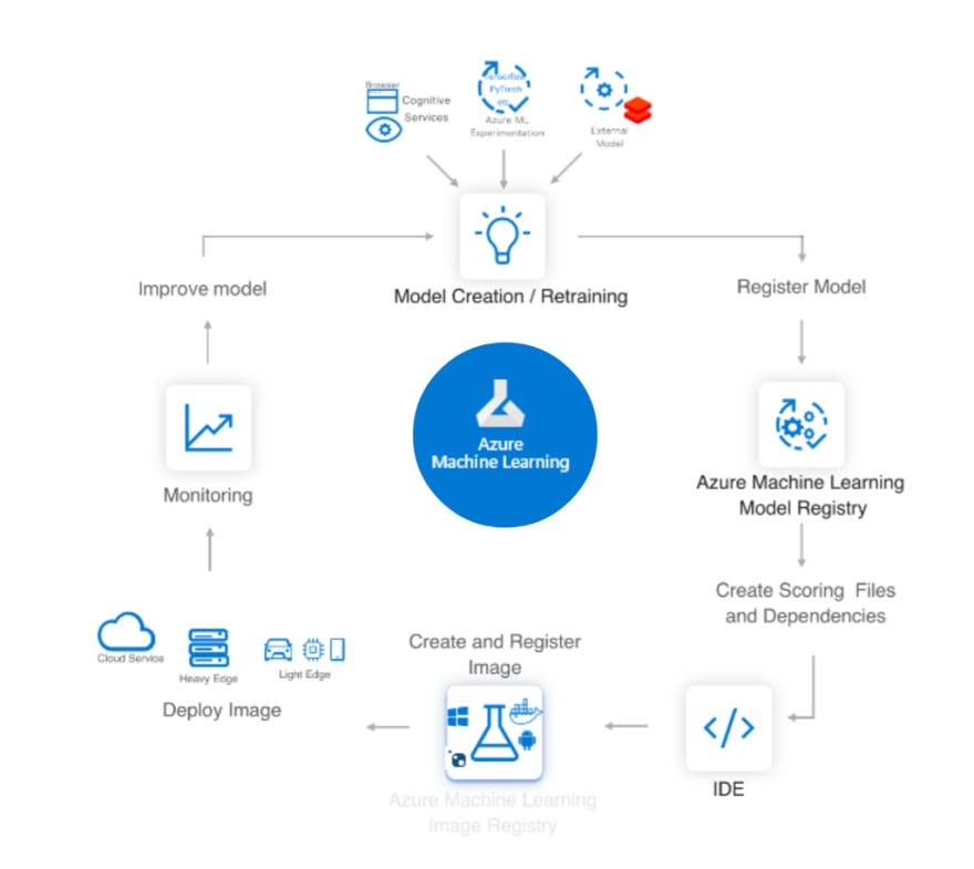
In summary, the scenario is the following one:

What About The R Community Engagement?

In the last 3 years Microsoft pushed a lot over the Azure ML Python SDK, making it a stable product and a first class citizen of the Azure cloud. But they seem to have forgotten all the R professionals who developed a huge amount of data science project all around the world.

We must not forget that in Analytics and Data Science the key of success of a project is to quickly try out a large number of analytical tools and find what’s the best one for the case in analysis. R was born for this reason. It has a lot of flexibility when you want to work with data and build some model, because it has tons of packages and easy of use visualization functionality. That’s why a lot of Analytics projects are developed using R by many statisticians and data scientists.

Fortunately in the last months Microsoft extended a hand to the R community, releasing a new project called Azure Machine Learning R SDK.

Can I Use R To Spin The Azure ML Wheels?

Starting from October 2019 Microsoft released a R interface for Azure Machine Learning SDK on GitHub. The idea behind this project is really straightforward. The Azure ML Python SDK is a way to simplify the access and the use of the Azure cloud storage and computation for machine learning purposes keeping the main code as the one a data scientist developed on its laptop.

Why not allow the Azure ML infrastructure to run also R code (using proper “cooked” Docker images) and let R data scientists call the Azure ML Python SDK methods using R functions?

The interoperability between Python and R is obtained thanks to reticulate. So, once the Python SDK module azureml is imported into any R environment using the import function, functions and other data within the azureml module can be accessed via the $ operator, like an R list.

Obviously, the machine hosting your R environment must have Python installed too in order to make the R SDK work properly.

Let’s start to configure your preferred environment.

Set Up A Development Environment For The R SDK

There are two option to start developing with the R SDK:

Using an Azure ML Compute Instance (the fastest way, but not the cheaper one!)
Using your machine (laptop, VM, etc.)

Set Up An Azure ML Compute Instance

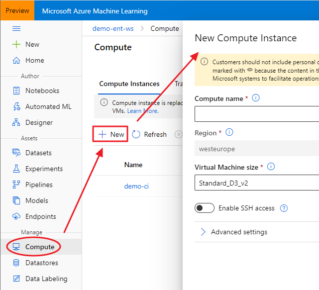
Once you created an Azure Machine Learning Workspace through the Azure portal (a basic edition is enough), you can access to the brand new Azure Machine Learning Studio. Under the Compute section, you can create a new Compute Instance, choosing its name and its sizing:

fig. 2 — Create an Azure ML Compute Instance

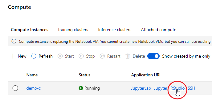
The advantage of using a Compute Instance is that the most used software and libraries by data scientists are already installed, including the Azure ML Python SDK and RStudio Server Open Source Edition. That said, once your Compute Instance is started, you can connect to RStudio using the proper link:

fig. 3 — Launch RStudio from a started Compute Intstance

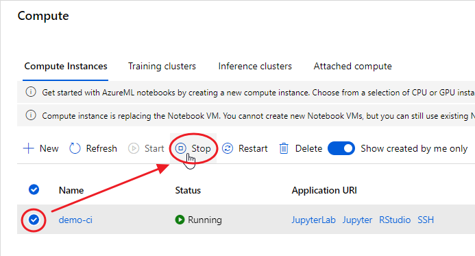
At the end of your experimentation, remember to shut down your Compute Instance, otherwise you’ll be charged according to the chosen plan:

Set Up Your Machine From Scratch

First of all you need to install the R engine from CRAN or MRAN. Then you could also install RStudio Desktop, the preferred IDE of R professionals.

The next step is to install Conda, because the R SDK needs to bind to the Python SDK through reticulate. If you really don’t need Anaconda for specific purposes, it’s recommended to install a lightweight version of it, Miniconda. During its installation, let the installer add the conda installation of Python to your PATH environment variable.

Install The R SDK

Open your RStudio, simply create a new R script (File → New File → R Script) and install the last stable version of Azure ML R SDK package (azuremlsdk) available on CRAN in the following way:

install.packages("remotes")
remotes::install_cran("azuremlsdk")

If you want to install the latest committed version of the package from GitHub (maybe because the product team has fixed an annoying bug), you can instead use the following function:

remotes::install_github('https://github.com/Azure/azureml-sdk-for-r')

During the installation you could get this error:

In this case, you just need to set the TZ environment variable with your preferred timezone:

Sys.setenv(TZ="GMT")

Then simply re-install the R SDK.

You may also be asked to update some dependent packages:

fig. 6 — Dependent packages to be updated

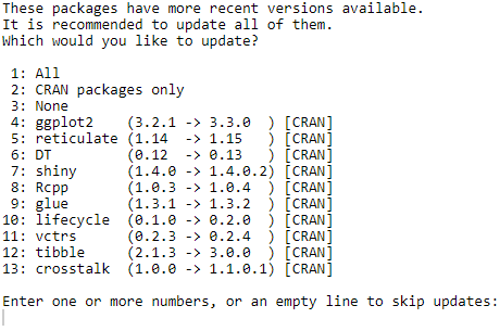
If you don’t have any requirement about dependencies in your project, it’s always better to update them all (put focus on the prompt in the console; press 1; press enter).

If you are on your Compute Instance and you get a warning like the following one:

fig. 7 — Warning about non-system installation of Python

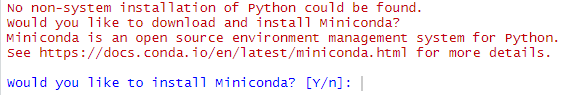
just put the focus on the console and press “n”, since the Compute Instance environment already has a Conda installation. Microsoft engineers are already investigating on this issue.

You need then to install the Azure ML Python SDK, otherwise your azuremlsdk R package won’t work. You can do that directly from RStudio thanks to an azuremlsdk function:

azuremlsdk::install_azureml(remove_existing_env = TRUE)

The remove_existing_env parameter set to TRUE will remove the default Azure ML SDK environment r-reticulate if previously installed (it’s a way to clean up a Python SDK installation).

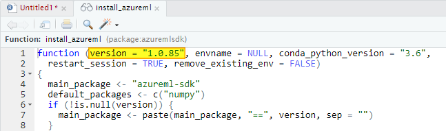
Just keep in mind that in this way you’ll install the version of the Azure ML Python SDK expected by your installed version of the azuremlsdk package. You can check what version you will install putting the cursor over the install_azureml function and visualizing the code definition clicking F2:

fig. 8 — install_azureml code definition

Sometimes there are new feature and fixes on the latest version of the Python SDK. If you need to install it, first check what version is available on this link:

fig. 9 — Azure ML Python SDK latest version

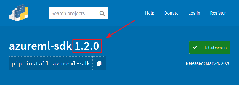
Then use that version number in the following code:

azuremlsdk::install_azureml(version = "1.2.0", remove_existing_env = TRUE)

Sometimes you may need to install an updated version of a single component of the Azure ML Python SDK to test, for example new features. Supposing you want to update the Azure ML Data Prep SDK, here the code you could use:

reticulate::py_install("azureml-dataprep==1.4.2", envname = "r-reticulate", pip = TRUE)

In order to check if the installation is working correctly, try this:

library(azuremlsdk)
get_current_run()

It should return something like this:

fig. 10 — Checking that azuremlsdk is correctly installed

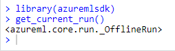
Great! You’re now ready to spin the Azure ML wheels using your preferred programming language: R!

Conclusions

After a long period during which Microsoft focused exclusively on Python SDK to enable data scientists to benefit from Azure computing and storage services, they recently released the R SDK too. This article focuses on the steps needed to install the Azure Machine Learning R SDK on your preferred environment.

Next articles will deal with the R SDK main capabilities.

R as learning tool: solving integrals

Integrals are so easy only math teachers could make them difficult.When I was in high school I really disliked math and, with hindsight, I would say it was just because of the the prehistoric teaching tools (when I saw this video I thought I’m not alone). I strongly believe that interaction CAUSES learning (I’m using “causes” here on purpose being quite aware of the difference between correlation and causation), practice should come before theory and imagination is not a skill you, as a teacher, could assume in your students. Here follows a short and simple practical explanation of integrals. The only math-thing I will write here is the following: f(x) = x + 7. From now on everything will be coded in R. So, first of all, what is a function? Instead of using the complex math philosophy let’s just look at it with a programming eye: it is a tool that takes something in input and returns something else as output. For example, if we use the previous tool with 2 as an input we get a 9. Easy peasy. Let’s look at the code:

# here we create the tool (called "f")
# it just takes some inputs and add it to 7
f <- function(x){x+7}

# if we apply it to 2 it returns a 9
f(2)
9

Then the second question comes by itself. What is an integral? Even simpler, it is just the sum of this tool applied to many inputs in a range. Quite complicated, let’s make it simpler with code:

# first we create the range of inputs
# basically x values go from 4 to 6 
# with a very very small step (0.01)
# seq stands for sequence(start, end, step)

x <- seq(4, 6, 0.01) 
x
4.00 4.01 4.02 4.03 4.04 4.05 4.06 4.07...

x[1]
4

x[2]
4.01

As you see, x has many values and each of them is indexed so it’s easy to find, e.g. the first element is 4 (x[1]). Now that we have many x values (201) within the interval from 4 to 6, we compute the integral.

# since we said that the integral is 
# just a sum, let's call it IntSum and 
# set it to the start value of 0
# in this way it will work as an accumulator

IntSum = 0

Differently from the theory in which the calculation of the integral produces a new non-sense formula (just kidding, but this seems to be what math teachers are supposed to explain), the integral does produce an output, i.e. a number. We find this number by summing the output of each input value we get from the tool (e.g. 4+7, 4.01+7, 4.02+7, etc) multiplied by the step between one value and the following (e.g. 4.01-4, 4.02-4.01, 4.03-4.02, etc). Let’s clarify this, look down here:

# for each value of x 
for(i in 2:201){
    
    # we do a very simple thing:
    # we cumulate with a sum
    # the output value of the function f 
    # multiplied by each steps difference
    
    IntSum = IntSum + f(x[i])*(x[i]-x[i-1])
    
    
    # So for example,  
    # with the first and second x values the numbers will be:
    #0.1101 = 0 + (4.01 + 7)*(4.01 - 4)
    
    # with the second and third:
    #0.2203 = 0.1101 + (4.02 + 7)*(4.02 - 4.01)
    
    # with the third and fourth:
    #0.3306 = 0.2203 + (4.03 + 7)*(4.03 - 4.02)
    
    # and so on... with the sum (integral) growing and growing
    # up until the last value
}

IntSum
24.01

Done! We have the integral but let’s have a look to the visualization of this because it can be represented and made crystal clear. Let’s add a short line of code to serve the purpose of saving the single number added to the sum each time. The reason why we decide to call it “bin” instead of, for example, “many_sum” will be clear in a moment.

# we need to store 201 calculation and we
# simply do what we did for IntSum but 201 times
bin = rep(0, 201)
bin
0 0 0 0 0 0 0 0 0 0 0 0 ...

Basically, we created a sort of memory to host each of the calculation as you see down here:

for (i in 2:201){
    
    # the sum as earlier
    IntSum = IntSum + f(x[i])*(x[i]-x[i-1])
    
    # overwrite each zero with each number
    bin[i] = f(x[i])*(x[i]-x[i-1])
}

IntSum
24.01

bin
0.0000 0.1101 0.1102 0.1103 0.1104 0.1105 ..

sum(bin)
24.01

Now if you look at the plot below you get the whole story: each bin is a tiny bar with a very small area and is the smallest part of the integral (i.e. the sum of all the bins).

# plotting them all
barplot(bin, names.arg=x)

This tells you a lot about the purpose of integral and the possibility of calculating areas of curvy surfaces. To have an idea of this just change the function f with, let’s say, sin(x) or log(x). What is happening? And what if you increase/decrease the number of bins? Have fun replicating the code changing some numbers and functions. Integrals should be clearer in the end. That’s all folks! #R #rstats #maRche #Rbloggers

This post is also shared in https://www.linkedin.com/in/roberto-palloni-6b224031/ and www.r-bloggers.com

“Print hello” is not enough. A collection of Hello world functions.

I guess I wrote my R “hello world!” function 7 or 8 years ago while approaching R for the first time. And it is too little to illustrate the basic syntax of a programming language for a working program to a wannabe R programmer. Thus, here follows a collection of basic functions that may help a bit more than the famed piece of code.

######################################################
############### Hello world functions ################
######################################################
##################################
# General info
fun <- function( arguments ) { body }


##################################
foo.add <- function(x,y){
  x+y
}

foo.add(7, 5)

----------------------------------

foo.above <- function(x){
  x[x>10]
}

foo.above(1:100)

----------------------------------

foo.above_n <- function(x,n){
  x[x>n]
}

foo.above_n(1:20, 12)

----------------------------------

foo = seq(1, 100, by=2)
foo.squared = NULL

for (i in 1:50 ) {
  foo.squared[i] = foo[i]^2
}

foo.squared

----------------------------------

a <- c(1,6,7,8,8,9,2)

s <- 0
for (i in 1:length(a)){
  s <- s + a[[i]]
}
s

----------------------------------

a <- c(1,6,7,8,8,9,2,100)

s <- 0
i <- 1
while (i <= length(a)){
  s <- s + a[[i]]
  i <- i+1
}
s

----------------------------------

FunSum <- function(a){
  s <- 0
  i <- 1
  while (i <= length(a)){
    s <- s + a[[i]]
    i <- i+1
  }
  print(s)
}

FunSum(a)

-----------------------------------

SumInt <- function(n){
  s <- 0
  for (i in 1:n){
    s <- s + i
  }
  print(s)  
}

SumInt(14)

-----------------------------------
# find the maximum
# right to left assignment
x <- c(3, 9, 7, 2)

# trick: it is necessary to use a temporary variable to allow the comparison by pairs of
# each number of the sequence, i.e. the process of comparison is incremental: each time
# a bigger number compared to the previous in the sequence is found, it is assigned as the
# temporary maximum
# Since the process has to start somewhere, the first (temporary) maximum is assigned to be
# the first number of the sequence

max <- x[1]
for(i in x){
  tmpmax = i
  if(tmpmax > max){
    max = tmpmax
  }
}

max

x <- c(-20, -14, 6, 2)
x <- c(-2, -24, -14, -7)

min <- x[1]
for(i in x){
  tmpmin = i
  if(tmpmin < min){
    min = tmpmin
  }
}

min

----------------------------------
# n is the nth Fibonacci number
# temp is the temporary variable

Fibonacci <- function(n){
  a <- 0
  b <- 1
  for(i in 1:n){
    temp <- b
    b <- a
    a <- a + temp
  }
  return(a)
}

Fibonacci(13)

----------------------------------
# R available factorial function
factorial(5)

# recursive function: ff
ff <- function(x) {
  if(x<=0) {
    return(1)
  } else {
    return(x*ff(x-1)) # function uses the fact it knows its own name to call itself
  }
}
ff(5)

----------------------------------

say_hello_to <- function(name){
  paste("Hello", name)
} 
say_hello_to("Roberto")

----------------------------------

foo.colmean <- function(y){
  nc <- ncol(y)
  means <- numeric(nc)
  for(i in 1:nc){
    means[i] <- mean(y[,i])
  }
  means
}

foo.colmean(airquality)

----------------------------------

foo.colmean <- function(y, removeNA=FALSE){
  nc <- ncol(y)
  means <- numeric(nc)
  for(i in 1:nc){
    means[i] <- mean(y[,i], na.rm=removeNA)
  }
  means
}

foo.colmean(airquality, TRUE)

----------------------------------

foo.contingency <- function(x,y){
  nc <- ncol(x)
  out <- list() 
  for (i in 1:nc){
    out[[i]] <- table(y, x[,i]) 
  }
  names(out) <- names(x)
  out
}

set.seed(123)
v1 <- sample(c(rep("a", 5), rep("b", 15), rep("c", 20)))
v2 <- sample(c(rep("d", 15), rep("e", 20), rep("f", 5)))
v3 <- sample(c(rep("g", 10), rep("h", 10), rep("k", 20)))

data <- data.frame(v1, v2, v3)

foo.contingency(data,v3)

That's all folks! #R #rstats #maRche #Rbloggers This post is also shared in LinkedIn and www.r-bloggers.com

Web data acquisition: from database to dataframe for data analysis and visualization (Part 4)

The previous post described how the deeply nested JSON data on fligths were parsed and stored in an R-friendly database structure. However, looking into the data, the information is not yet ready for statistical analysis and visualization and some further processing is necessary before extracting insights and producing nice plots. In the parsed batch, it is clearly visible the redundant structure of the data with the flight id repeted for each segment of each flight. This is also confirmed with the following simple check as the rows of the dataframe are more than the unique counts of the elements in the id column.

dim(data_items)
[1] 397  15

length(unique(data_items$id))
201

# real time changes of data could produce different results

This implies that the information of each segment of each flight has to be aggregated and merged in a dataset as single observations of a statistical analysis between, for example, price and distance. First, a unique primary key for each observation has to be used as reference variable to uniquely identify each element of the dataset.

library(plyr) # sql like functions
library(readr) # parse numbers from strings
 
data_items <- data.frame(data_items)
 
# id (primary key)
data <- data.frame(unique(data_items$id))
colnames(data) <- c('id')
 
# n° of segment
n_segment <- aggregate(data_items['segment.id'], by=data_items['id'], length)
data <- join(data, n_segment, by='id', type='left', match='first') # sql left join
# mileage
mileage <- aggregate(data_items['segment.leg.mileage'], by=data_items['id'], sum)
data <- join(data, mileage, by='id', type='left', match='first') # sql left join
# price
price <- data.frame('id'=data_items$id, 'price'=parse_number(data_items$saleTotal))
data <- join(data, price, by='id', type='left', match='first') # sql left join
# dataframe
colnames(data) <- c('id','segment', 'mileage', 'price')
head(data)

The aggregation of mileage and price using the unique primary key allows to set up a dataframe ready for statistical analysis and data visualization. Current data tells us that there is a maximum of three segments in the connection between FCO and LHR with a minimum price of around EUR 122 and a median around EUR 600.


# descriptive statistics
summary(data)
 
 
# histogram price & distance
g1 <- ggplot(data, aes(x=price)) + 
  geom_histogram(bins = 50) +  
  ylab("Distribution of the Price (EUR)") +
  xlab("Price (EUR)") 
 
g2 <- ggplot(data, aes(x=mileage)) + 
  geom_histogram(bins = 50) +  
  ylab("Distribution of the Distance") +
  xlab("Distance (miles)")
 
grid.arrange(g1, g2)
# price - distance relationship
s0 <- ggplot(data = data, aes(x = mileage, y = price)) +
    geom_smooth(method = "lm", se=FALSE, color="black") +
    geom_point() + labs(x = "Distance in miles", y = "Price (EUR)")
s0 <- ggMarginal(s0, type = "histogram", binwidth = 30)
s0

Of course, plenty of other analysis and graphical representations using flights features are possible given the large set of variables available in QPX Express API and the availability of data in real time.

To conclude the 4-step (flight) trip from data acquisition to data analysis, let's recap the most important concepts described in each of the post: 1) Client-Server connection 2) POST request in R 3) Data parsing and structuring 4) Data analysis and visualization

That's all folks! #R #rstats #maRche #json #curl #qpxexpress #Rbloggers This post is also shared in www.r-bloggers.com

Web data acquisition: parsing json objects with tidyjson (Part 3)

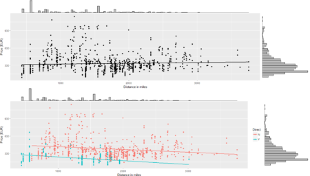
The collection of example flight data in json format available in part 2, described the libraries and the structure of the POST request necessary to collect data in a json object. Despite the process generated and transferred locally a proper response, the data collected were neither in a suitable structure for data analysis nor immediately readable. They appears as just a long string of information nested and separated according to the JavaScript object notation syntax. Thus, to visualize the deeply nested json object and make it human readable and understandable for further processing, the json content could be copied and pasted in a common online parser. The tool allows to select each node of the tree and observe the data structure up to the variables and data of interest for the statistical analysis. The bulk of the relevant information for the purpose of the analysis on flight prices are hidden in the tripOption node as shown in the following figure (only 50 flight solutions were requested).

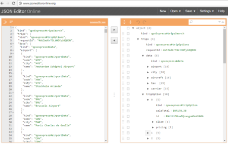
However, looking deeply into the object, several other elements are provided as the distance in mile, the segment, the duration, the carrier, etc. The R parser to transform the json structure in a usable dataframe requires the dplyr library for using the pipe operator (%>%) to streamline the code and make the parser more readable. Nevertheless, the library actually wrangling through the lines is tidyjson and its powerful functions:

enter_object: enters and dives into a data object;
gather_array: stacks a JSON array;
spread_values: creates new columns from values assigning specific type (e.g. jstring, jnumber).

library(dplyr) # for pipe operator %>% and other dplyr functions library(tidyjson) # https://cran.r-project.org/web/packages/tidyjson/vignettes/introduction-to-tidyjson.html data_items <- datajson %>% spread_values(kind = jstring("kind")) %>% spread_values(trips.kind = jstring("trips","kind")) %>% spread_values(trips.rid = jstring("trips","requestId")) %>% enter_object("trips","tripOption") %>% gather_array %>% spread_values( id = jstring("id"), saleTotal = jstring("saleTotal")) %>% enter_object("slice") %>% gather_array %>% spread_values(slice.kind = jstring("kind")) %>% spread_values(slice.duration = jstring("duration")) %>% enter_object("segment") %>% gather_array %>% spread_values( segment.kind = jstring("kind"), segment.duration = jnumber("duration"), segment.id = jstring("id"), segment.cabin = jstring("cabin")) %>% enter_object("leg") %>% gather_array %>% spread_values( segment.leg.aircraft = jstring("aircraft"), segment.leg.origin = jstring("origin"), segment.leg.destination = jstring("destination"), segment.leg.mileage = jnumber("mileage")) %>% select(kind, trips.kind, trips.rid, saleTotal,id, slice.kind, slice.duration, segment.kind, segment.duration, segment.id, segment.cabin, segment.leg.aircraft, segment.leg.origin, segment.leg.destination, segment.leg.mileage) head(data_items) kind trips.kind trips.rid saleTotal 1 qpxExpress#tripsSearch qpxexpress#tripOptions UnxCOx4nKIcIOpRiG0QBOe EUR178.38 2 qpxExpress#tripsSearch qpxexpress#tripOptions UnxCOx4nKIcIOpRiG0QBOe EUR178.38 3 qpxExpress#tripsSearch qpxexpress#tripOptions UnxCOx4nKIcIOpRiG0QBOe EUR235.20 4 qpxExpress#tripsSearch qpxexpress#tripOptions UnxCOx4nKIcIOpRiG0QBOe EUR235.20 5 qpxExpress#tripsSearch qpxexpress#tripOptions UnxCOx4nKIcIOpRiG0QBOe EUR248.60 6 qpxExpress#tripsSearch qpxexpress#tripOptions UnxCOx4nKIcIOpRiG0QBOe EUR248.60 id slice.kind slice.duration 1 ftm7QA6APQTQ4YVjeHrxLI006 qpxexpress#sliceInfo 510 2 ftm7QA6APQTQ4YVjeHrxLI006 qpxexpress#sliceInfo 510 3 ftm7QA6APQTQ4YVjeHrxLI009 qpxexpress#sliceInfo 490 4 ftm7QA6APQTQ4YVjeHrxLI009 qpxexpress#sliceInfo 490 5 ftm7QA6APQTQ4YVjeHrxLI007 qpxexpress#sliceInfo 355 6 ftm7QA6APQTQ4YVjeHrxLI007 qpxexpress#sliceInfo 355 segment.kind segment.duration segment.id segment.cabin 1 qpxexpress#segmentInfo 160 GixYrGFgbbe34NsI COACH 2 qpxexpress#segmentInfo 235 Gj1XVe-oYbTCLT5V COACH 3 qpxexpress#segmentInfo 190 Grt369Z0shJhZOUX COACH 4 qpxexpress#segmentInfo 155 GRvrptyoeTfrSqg8 COACH 5 qpxexpress#segmentInfo 100 GXzd3e5z7g-5CCjJ COACH 6 qpxexpress#segmentInfo 105 G8axcks1R8zJWKrN COACH segment.leg.aircraft segment.leg.origin segment.leg.destination segment.leg.mileage 1 320 FCO IST 859 2 77W IST LHR 1561 3 73H FCO ARN 1256 4 73G ARN LHR 908 5 319 FCO STR 497 6 319 STR LHR 469 Data are now in an R-friendly structure despite not yet ready for analysis. As can be observed from the first rows, each record has information on a single segment of the flight selected. A further step of aggregation using some SQL is needed in order to end up with a dataframe of flights data suitable for statistical analysis. Next up, the aggregation, some data analysis and data visualization to complete the journey through the web data acquisition using R. #R #rstats #maRche #json #curl #tidyjson #Rbloggers This post is also shared in www.r-bloggers.com and LinkedIn