
Integrals are so easy only math teachers could make them difficult.When I was in high school I really disliked math and, with hindsight, I would say it was just because of the the prehistoric teaching tools (when I saw this video I thought I’m not alone). I strongly believe that interaction CAUSES learning (I’m using “causes” here on purpose being quite aware of the difference between correlation and causation), practice should come before theory and imagination is not a skill you, as a teacher, could assume in your students. Here follows a short and simple practical explanation of integrals. The only math-thing I will write here is the following: f(x) = x + 7. From now on everything will be coded in R. So, first of all, what is a function? Instead of using the complex math philosophy let’s just look at it with a programming eye: it is a tool that takes something in input and returns something else as output. For example, if we use the previous tool with 2 as an input we get a 9. Easy peasy. Let’s look at the code:
# here we create the tool (called "f")
# it just takes some inputs and add it to 7
f <- function(x){x+7}

# if we apply it to 2 it returns a 9
f(2)
9
Then the second question comes by itself. What is an integral? Even simpler, it is just the sum of this tool applied to many inputs in a range. Quite complicated, let’s make it simpler with code:
# first we create the range of inputs
# basically x values go from 4 to 6
# with a very very small step (0.01)
# seq stands for sequence(start, end, step)
x <- seq(4, 6, 0.01)
x
4.00 4.01 4.02 4.03 4.04 4.05 4.06 4.07...

x[1]
4

x[2]
4.01
As you see, x has many values and each of them is indexed so it’s easy to find, e.g. the first element is 4 (x[1]). Now that we have many x values (201) within the interval from 4 to 6, we compute the integral.
# since we said that the integral is
# just a sum, let's call it IntSum and
# set it to the start value of 0
# in this way it will work as an accumulator
IntSum = 0Differently from the theory in which the calculation of the integral produces a new non-sense formula (just kidding, but this seems to be what math teachers are supposed to explain), the integral does produce an output, i.e. a number. We find this number by summing the output of each input value we get from the tool (e.g. 4+7, 4.01+7, 4.02+7, etc) multiplied by the step between one value and the following (e.g. 4.01-4, 4.02-4.01, 4.03-4.02, etc). Let’s clarify this, look down here:
# for each value of x
for(i in 2:201){

    # we do a very simple thing:
    # we cumulate with a sum
    # the output value of the function f
    # multiplied by each steps difference

    IntSum = IntSum + f(x[i])*(x[i]-x[i-1])


    # So for example,
    # with the first and second x values the numbers will be:
    #0.1101 = 0 + (4.01 + 7)*(4.01 - 4)

    # with the second and third:
    #0.2203 = 0.1101 + (4.02 + 7)*(4.02 - 4.01)

    # with the third and fourth:
    #0.3306 = 0.2203 + (4.03 + 7)*(4.03 - 4.02)

    # and so on... with the sum (integral) growing and growing
    # up until the last value
}

IntSum
24.01
Done! We have the integral but let’s have a look to the visualization of this because it can be represented and made crystal clear. Let’s add a short line of code to serve the purpose of saving the single number added to the sum each time. The reason why we decide to call it “bin” instead of, for example, “many_sum” will be clear in a moment.
# we need to store 201 calculation and we
# simply do what we did for IntSum but 201 times
bin = rep(0, 201)
bin
0 0 0 0 0 0 0 0 0 0 0 0 ...
Basically, we created a sort of memory to host each of the calculation as you see down here:
for (i in 2:201){
# the sum as earlier
IntSum = IntSum + f(x[i])*(x[i]-x[i-1])
# overwrite each zero with each number
bin[i] = f(x[i])*(x[i]-x[i-1])
}
IntSum
24.01
bin
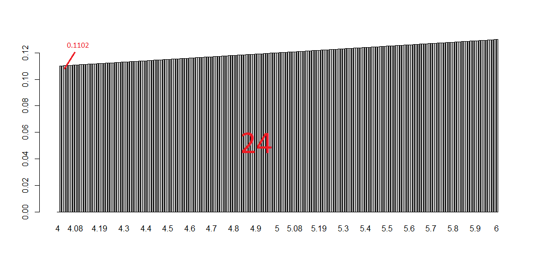
0.0000 0.1101 0.1102 0.1103 0.1104 0.1105 ..
sum(bin)
24.01
Now if you look at the plot below you get the whole story: each bin is a tiny bar with a very small area and is the smallest part of the integral (i.e. the sum of all the bins).
# plotting them all
barplot(bin, names.arg=x)
This post is also shared in https://www.linkedin.com/
Primo
Thanks, very clear explanation.
I enjoyed your recent post on R and integrals. How can I use the post to integrate the following and get a rough image: x=60/y=0, x=48/y=2.5, x=36/y=4.5, x=24/y=6, and x=12/y=5.5. These are actual measurements, and I can create the equation and look for the anti-derivative. But I was hoping that with your post this could be done more efficiently in R and be used to check my work.
Thanks for your time,
-T
I don’t really understand your criticisms of math teachers or the theory of integration. The standard approach to teaching integrals follows along the lines of what you have done: break up the domain into bins and compute the sum (Riemann sum approximation). Some natural questions to ask are “how does the choice of bins effect the sum?”, “if the bin widths get smaller, do the sums approach a fixed number?”, “does this process work for every function?”, “is there an analytical (i.e. formulaic) way to do this for some functions?”, etc. Answering these questions leads to the theory of Riemann integration and the undergrad techniques for computing anti-derivatives of some elementary functions. Bad teachers may not motivate calculus/analysis well, but there are bad teachers in every field. There are very many well-written books that properly motivate this topic.
I agree with Chris. It all depends on how the subject is taught. A much neglected text is Richard Courant’s “Differential and Integral Calculus” which I think is still in print. Frankly, calculus has been so dumbed down that even the mathematically gifted find many modern texts hard to follow. So look for older ones. Sure, they don’t have the neat pictures and graphics but they were better thought out.
Courant was a great advocate of applied math and went to great lengths to illustrate math through practical examples. There’s a YouTube of him illustrating something about partial differential equations and boundary conditions using soap bubbles and wire. Also check out some of Peter Lax’s work. Though a great mathematician, he has worked a lot on math education and has always loved teaching beginners.
As for R. It amazes me how many–even among the young–are still using for loops. One of the great advantages of R is that these are virtually unnecessary. Here’s what you did without using a loop. Also, I included coding for unequally spaced partitions as well as equally spaced ones. The Riemann sum is absolutely simple and a direct expression of the formula–something lacking when one uses a loop:
x=c(4,sort(runif(180,4,6)),6) # Generate an unequally spaced partition
x=seq(4,6,.1) # Generate an equally spaced partition (one or the other)
dx=diff(x) # We lose a value when taking first differences
xt<-x[-1] # drop first value of x (sum from i=2 to i=n)
sum(f(xt)*dx) # approximate value of the integral
IntSum=c(0,cumsum(f(xt)*dx)) # form the cumulative sum (when plotted will look like the antiderivative of x+7)