by Jerry Tuttle
I would like to share some thoughts about outliers and domain knowledge.
One of the common steps during the data exploration stage is the search for outliers. Some analysis methods such as regression are very sensitive to outliers. As an example of sensitivity, in the following data (10,10) is an outlier. Including the outlier produces a regression line y = .26 + .91x, while excluding the outlier produces the very different regression line y = 2.
x <- c(1,1,1,2,2,2,3,3,3,10)
y <- c(1,2,3,1,2,3,1,2,3,10)
df <- data.frame(cbind(x,y))
lm(y ~ x, df)
plot(x,y, pch=16)
abline(lm(y ~ x, df)
Statistics books sometimes define an outlier as being outside the range of Q1 ± 1.5IQR or Q1 ± 3IQR, where Q1 is the lower quartile (25th percentile value), Q3 is the upper quartile (75th percentile value), and the interquartle range IQR = Q3 – Q1.
What does one do with an outlier? It could be bad data. It is pretty unlikely that there is a graduate student who is age 9, but we don’t know whether the value should be 19 (very rare, but possible), or 29 (likely), or 39 or more (not so rare). If we have the opportunity to ask the owner of the data, perhaps we can get the value corrected. More likely is we can not ask the owner. We can delete the entire observation, or we can pretend to correct the value with a mode or median value or a judgmental value.
Perhaps the outlier is not bad data but rather just an unusual value. In a portfolio of property or liability insurance claims, the distribution is often positively skewed (mean greater than mode, a long tail to the positive side of the mode). Most claims are small, but occasionally there is that one enormous claim. What does one do with that outlier value? Some authors consider data science to be the Venn diagram intersection among math/statistics, computer science, and domain knowledge (see for example Drew Conway, in drewconway.com/zia/2013/3/26/the-data-science-venn-diagram). If the data scientist is not the domain expert, he or she should consult with one. With insurance claims there are several possibilities. One is that the enormous claim is one that is unlikely to reoccur for any number of reasons. Hopefully there will never be another September 11 type destruction of two World Trade Center buildings owned by a single owner. Another example is when the insurance policy terms are revised to literally prohibit a specific kind of claim in the future. Another possibility is that the specific claim is unlikely to reoccur (the insurance company stopped insuring wheelchairs, so there won’t be another wheelchair claim), but that claim is representative of another kind of claim that is likely to occur. In this case, the outlier should not be deleted. One author has said it takes Solomon-like wisdom to discern which possibility to believe.
An interesting example of outliers occurs with sports data. For many reasons, US major league baseball player statistics have changed over the years. There are more great home run seasons nowadays than decades ago, but there are fewer great batting average seasons. Baseball fanatics know the last .400 hitter (40% ratio of hits divided by at bats over the entire season) was Ted Williams in 1941. If we have 80 years of baseball data and we are predicting the probability of another .400 hitter, we would predict close to zero. It’s possible, but extremely unlikely, right? Actually no. Assuming there will still be a shortened season in 2020, a decision that may change, this author is willing to forecast that there will be a .400 hitter in a shortened season. This is due to the theory that batters need less time in spring training practice to be at full ability than pitchers, and it is easier to achieve .400 in a small number of at bats earlier in the season when the pitchers are not at full ability. This is another example of domain expertise as a lifetime baseball fan.
Category: R
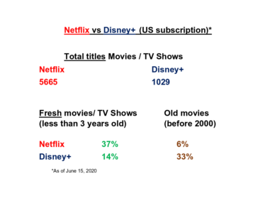
Netflix vs Disney+. Who has more fresh titles?
“Let`s shift to Disney+”, said my wife desperately browsing Netflix on her phone. “Netflix has much more fresh content” I argued. And…I realized I need numbers to close these family debates…
I choose “2018 and later” criteria as “fresh” and “1999 and earlier” as “old”. Those criteria are not strict but I needed certainty to have completely quantified arguments to keep my Netflix on the family throne.
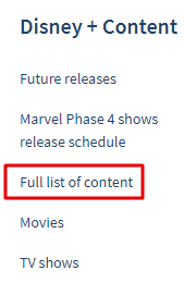
Since I did not find such numbers on both streaming services websites I decided to scrape full lists of movies and TV shows and calculate % of “fresh” / “old” movies in entire lists. Likely, there are different websites listing all movies and TV shows both on Disney+ and Netflix and updating them daily. I choose one based on popularity (I checked it both with Alexa and Similar Web) and its architecture making my scraping job easy and predictable.
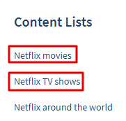
For Netflix content our source website does not have single page so I scraped movies and TV shows separately.
Since I did not find such numbers on both streaming services websites I decided to scrape full lists of movies and TV shows and calculate % of “fresh” / “old” movies in entire lists. Likely, there are different websites listing all movies and TV shows both on Disney+ and Netflix and updating them daily. I choose one based on popularity (I checked it both with Alexa and Similar Web) and its architecture making my scraping job easy and predictable.
library (tidyverse)
library (rvest)
disney0 <- read_html("https://www.finder.com/complete-list-disney-plus-movies-tv-shows-exclusives/")
Locate proper CSS element using Selector Gadget disney_year_0 <- html_nodes(disney0, 'td:nth-child(2)') disney_year <- html_text (disney_year_0, trim=TRUE) # list of release years for every title length (disney_year) #1029Now, let`s create frequency table for each year of release
disney_year_table <- as.data.frame (sort (table (disney_year), decreasing = TRUE), stringsAsFactors = FALSE)
colnames (disney_year_table) <- c('years', 'count')

glimpse (disney_year_table)
Rows: 89 Columns: 2 $ years  "2019", "2017", "2016", "2018", "2015", "2011", "2014", "2012", "2010", "200... $ count  71, 58, 48, 40, 36, 35, 35, 34, 31, 28, 28, 27, 27, 25, 24, 24, 23, 23, 21,
Finally, count ‘fresh’ and 'old' % in entire Disney+ offer
disney_year_table$years <- disney_year_table$years %>% as.numeric ()

fresh_disney_years <- disney_year_table$years %in% c(2018:2020)
fresh_disney_num <- paste (round (sum (disney_year_table$count[fresh_disney_years]) / sum (disney_year_table$count)*100),'%')

old_disney_years <- disney_year_table$years < 2000
old_disney_num <- paste (round (sum (disney_year_table$count[old_disney_years]) / sum (disney_year_table$count)*100),'%')
So, I`ve got roughly 14% “fresh” and 33% “old” movie on Disney+. Let`s see the numbers for Netflix.
For Netflix content our source website does not have single page so I scraped movies and TV shows separately.
#movies
netflix_mov0 <- read_html("https://www.finder.com/netflix-movies/")
netflix_mov_year_0 <- html_nodes(netflix_mov0, 'td:nth-child(2)')
netflix_mov_year <- tibble (html_text (netflix_mov_year_0, trim=TRUE))
colnames (netflix_mov_year) <- "year"

#TV shows
netflix_tv0 <- read_html("https://www.finder.com/netflix-tv-shows/")
netflix_tv_year_0 <- html_nodes(netflix_tv0, 'td:nth-child(2)')
netflix_tv_year <- tibble (html_text (netflix_tv_year_0, trim=TRUE))
colnames (netflix_tv_year) <- "year"
Code for final count of the at Neflix ‘fresh’ and ‘old’ movies / TV shows portions is almost the same as for Disney
netflix_year <- rbind (netflix_mov_year, netflix_tv_year)
nrow (netflix_year)
netflix_year_table <- as.data.frame (sort (table (netflix_year), decreasing = TRUE), stringsAsFactors = FALSE) colnames (netflix_year_table) <- c('years', 'count')

glimpse (netflix_year_table)
Rows: 68
Columns: 2
$ years  2018, 2019, 2017, 2016, 2015, 2014, 2020, 2013, 2012, 2010,
$ count  971, 882, 821, 653, 423, 245, 198, 184, 163, 127, 121, 108,
Count 'fresh' and 'old' % in entire offer
netflix_year_table$years <- netflix_year_table$years %>% as.numeric ()

fresh_netflix_years <- netflix_year_table$years %in% c(2018:2020)
fresh_netflix_num <- paste (round (sum (netflix_year_table$count[fresh_netflix_years]) / sum (netflix_year_table$count)*100),'%')

old_netflix_years <- netflix_year_table$years < 2000
old_netflix_years <- na.omit (old_netflix_years)
old_netflix_num <- paste (round (sum (netflix_year_table$count[old_netflix_years]) / sum (netflix_year_table$count)*100),'%')
So, finally, I can build my arguments based on numbers, freshly baked and bold
Version 0.1.4 of nnlib2Rcpp: a(nother) R package for Neural Networks
For anyone interested, a new version (v.0.1.4) of nnlib2Rcpp is available on GitHub. It can be installed the usual way for packages on GitHub:
Furthermore, a new “NN” module (NN-class) has been added to version 0.1.4, that allows the creation of custom NNs using predefined components, and manipulation of the network and its components from R. It also provides a fixed procedure for defining new NN component types (layers, nodes, sets of connections etc) which can then be used in the module (some familiarity with C++ is required).
The “NN” (aka NN-class) provides methods for handling the NN, such as: add_layer, add_connection_set, create_connections_in_sets, connect_layers_at, fully_connect_layers_at, add_single_connection, input_at, encode_at, encode_all, recall_at, recall_all, get_output_from, get_input_at, get_weights_at, print, outline.
A (rather useless and silly) example of using the “NN” module follows:
library(devtools)
install_github("VNNikolaidis/nnlib2Rcpp")
nnlib2Rcpp is an R package containing a number of Neural Network (NN) implementations. The NNs are implemented in C++ (using nnlib2 C++ class library) and are interfaced with R via Rcpp package (which is required). The package currently includes versions of Back-Propagation, Autoencoder, Learning Vector Quantization (unsupervised and supervised) and simple Matrix-Associative-Memory neural networks. Functions and modules for directly using these models from R are provided.Furthermore, a new “NN” module (NN-class) has been added to version 0.1.4, that allows the creation of custom NNs using predefined components, and manipulation of the network and its components from R. It also provides a fixed procedure for defining new NN component types (layers, nodes, sets of connections etc) which can then be used in the module (some familiarity with C++ is required).
The “NN” (aka NN-class) provides methods for handling the NN, such as: add_layer, add_connection_set, create_connections_in_sets, connect_layers_at, fully_connect_layers_at, add_single_connection, input_at, encode_at, encode_all, recall_at, recall_all, get_output_from, get_input_at, get_weights_at, print, outline.
A (rather useless and silly) example of using the “NN” module follows:
# (1.A) create new 'NN' object:
n <- new("NN")

# (1.B) Add topology components:
# 1. add a layer of 4 generic nodes:
n$add_layer("generic",4)
# 2. add (empty) set for connections that pass data unmodified:
n$add_connection_set("pass-through")
# 3. add another layer of 2 generic nodes:
n$add_layer("generic",2)
# 4. add (empty) set for connections that pass data * weight:
n$add_connection_set("wpass-through")
# 5. add a layer of 1 generic node:
n$add_layer("generic",1)
# Create actual connections in sets,w/random initial weights in [0,1]:
n$create_connections_in_sets(0,1)
# Optionally, show an outline of the topology:
n$outline()

# (1.C) use the network.
# input some data, and run create output for it:
n$input_at(1,c(10,20,30,40))
n$recall_all(TRUE)
# the final output:
n$get_output_from(5)

# (1.D) optionally, examine the network:
# the input at first layer at position 1:
n$get_input_at(1)
# Data is passed unmodified through connections at position 2,
# and (by default) summed together at each node of layer at 3.
# Final output from layer in position 3:
n$get_output_from(3)
# Data is then passed multiplied by the random weights through
# connections at position 4. The weights of these connections:
n$get_weights_at(4)
# Data is finally summed together at the node of layer at position 5,
# producing the final output, which (again) is:
n$get_output_from(5)
The next example, creates a simple MAM using the "NN" (NN-class) module:
# (2.A) Create the NN and its components:

m <- new( "NN" )
m$add_layer( "generic" , 4 )
m$add_layer( "generic" , 3 )
m$fully_connect_layers_at(1, 2, "MAM", 0, 0)

# (2.B) Use it to store iris species:

iris_data    <- as.matrix( scale( iris[1:4] ) )
iris_species <- as.integer( iris$Species )
for(r in 1:nrow( iris_data ) )
{
    x <- iris_data[r,]
    z <- rep( -1, 3 )
    z [ iris_species[r] ] <- 1
    m$input_at( 1, x )
    m$input_at( 3, z )
    m$encode_all( TRUE )
}

# (2.C) Attempt to recall iris species:

recalled_ids <- NULL;
for(r in 1:nrow(iris_data))
{
    x <- iris_data[r,]
    m$input_at( 1, x )
    m$recall_all( TRUE )
    z <- m$get_output_from( 3 )
    recalled_ids <- c( recalled_ids, which.max ( z ) )
}

plot(iris_data, pch=recalled_ids)
Hopefully the collection of predefined components will expand (and any contribution of components is welcomed). MultiNav: anomaly detection and interactive visualization with multivariate data.
In statistical process control (SPC), a.k.a. anomaly-detection, one compares some statistic to its “in control” distribution. Many statistical and BI software suits (e.g. Tableau, PowerBI) can do SPC. Almost all of these, however, focus on univariate processes, which are easier to visualize and discuss than multivariate processes.
The purpose of our Multinav package is to ingest multivariate data streams, compute multivariate summaries, and allow us to query the data interactively when an anomaly is detected.
In the following example we look into an agricultural IoT use-case, and try to detect sensors with anomalous readings. The data consists of hourly measurements, during 5 days, of the girth of 100 avocado trees. For each such tree, an anomaly score is computed using four variation of Hotelling’s T2 statistic. The full details are available in the official documentation.
This one line of code will produce the following dashboard:
Crucially for our purposes, this dashboard is interactive. Charts are linked so that one may hover over a particular point, and it will light in all panels (JMP and S+ style). Hovering over a point will also draw the raw evolution of the measurement in time and compare it to the group via a functional boxplot.
There is a lot more that MultiNav can do. The details can be found in the inline-help, and the official documentation. For the purpose of this blog, we merely summarize the reasons we find Multinav very useful:
1. Interactive visualizations that link anomaly score with raw data.
2. Functional boxplot for querying the source of the anomalies.
3. Out-of-the-box multivariate scoring functions, with the possibility of extension by the user.
4. The interactive component are embeddable in Shiny apps, for a full blown interactive dashboard.
The purpose of our Multinav package is to ingest multivariate data streams, compute multivariate summaries, and allow us to query the data interactively when an anomaly is detected.
In the following example we look into an agricultural IoT use-case, and try to detect sensors with anomalous readings. The data consists of hourly measurements, during 5 days, of the girth of 100 avocado trees. For each such tree, an anomaly score is computed using four variation of Hotelling’s T2 statistic. The full details are available in the official documentation.
This one line of code will produce the following dashboard:
MultiNav(data, type = "scores", xlbl="Date id")
Crucially for our purposes, this dashboard is interactive. Charts are linked so that one may hover over a particular point, and it will light in all panels (JMP and S+ style). Hovering over a point will also draw the raw evolution of the measurement in time and compare it to the group via a functional boxplot.
There is a lot more that MultiNav can do. The details can be found in the inline-help, and the official documentation. For the purpose of this blog, we merely summarize the reasons we find Multinav very useful:
1. Interactive visualizations that link anomaly score with raw data.
2. Functional boxplot for querying the source of the anomalies.
3. Out-of-the-box multivariate scoring functions, with the possibility of extension by the user.
4. The interactive component are embeddable in Shiny apps, for a full blown interactive dashboard.
springerQuarantineBooksR: Download all books made available by Springer during the COVID-19 quarantine!
Following
this recent blog post. I’d like to share a project that downloads all these books in R! It is called springerQuarantineBooksR. You can check it out in this link.
How to measure movies vocabulary and display results in nice tables using tidytext and gt packages. Movies text analysis. Part 2.
My primary goal was to research popular movies vocabulary – words all those heroes actually saying to us and put well known movies onto the scale from the ones with the widest lexicon down to below average range despite possible crowning by IMDB rating, Box Office revenue or number / lack of Academy Awards.
Main unit of analysis is Number of unique words per 1000 which says about how WIDE the vocabulary of each movie / TV show is. I saw and personally made similar analysis for literature, music or web content but never for real top movies texts, not scripts.
This post is the 2nd Part of the Movies text analysis and covers analysis itself and displaying results in nice looking tables using gt package. Part 1, previously published on R-Bloggers, covers preparation stage and movie texts cleaning using textclean package.
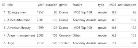
I created CSV file featuring movies:
Resulting table will be plugged with three more parameters needed to be calculated.
The same for ten least wordy movies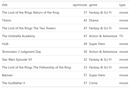
Only Reality Show I added as control value is obvious outlier. While the most silent are well known epic movies. We will explore gt package more deep a later. Now, let`s check the range for Total Number of words
5981 8619 10311 10815 12467 18710
I wish all of them were exact 10,000 words length. Or any other but equal length for all movies. Real life is not so round. Unlike music vocabulary, we cannot take "99.7 songs" to have the same length for every peer. Why we need that? We cannot properly compare Number of unique words within different pieces of text unless they all are the same length. Any one sentence has up to 100% words uniqueness, 100 sentences - up to 50%. Any entire movie – much less due to marginal saturation e.g. usage the words we already used.
Before we solve this problem we should lemmatize clean text.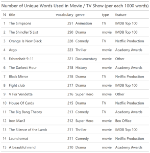
And we can easily save the table as graphical output.
We can change cells and text colors and even make it conditional (for instance, only ‘type == TV’).
That`s it for tables and for Part 2 of my Movies text analysis. In Part 3 I plan to use ggplot2 to visualize and compare how wide vocabulary is within iconic movies, different genres, Movies vs TV Shows, IMDB TOP 100 vs Box Office All Time Best etc. See ya.
Movies_prep <- read_csv("R/movies/Movies_prep.csv")
Movies_prep [1:5,]
Resulting table will be plugged with three more parameters needed to be calculated.
- Number of words (for entire movie).
- Words per minute (Number of words / Movie length).
- Vocabulary (Number of unique words per 1000 words).
library (tidyverse)
library (tidytext)
library (textstem)
library (gt)
Bind clean text (described in Movies text analysis. Part 1) to the titles
movies_ <- select (Movies_prep, title = title)
movies_bind <- cbind (movies_, text)
Let`s use tidytext package to Unnest text to words
movies_words <- unnest_tokens (movies_bind, word, text)Simply calculate nwords and words per minute for each movie
title_ <- movies_bind$title
movies_nword <- function (i){movies_nwords1<- movies_words %>% filter (title==i) %>% nrow ()
movies_nwords1}
movies_nwords <- sapply (title_, movies_nword)

Movies_prep1 <-  Movies_prep %>% mutate (words = movies_nwords, wpminute = round (movies_nwords/duration))
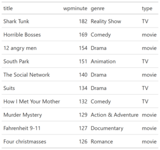
Let`s look at the Words per minute parameter first.wpm_summary <- Movies_prep1$wpminute %>% summary ()wpm_summary Min. 1st Qu. Median Mean 3rd Qu. Max. 37.00 66.00 80.00 85.89 104.00 182.00 Let`s check ten most wordy movies in our dataset
Movies_prep1_GT <- Movies_prep1 %>% select (title, wpminute, genre, type)
Movies_preptop_GT <- Movies_prep1_GT %>% arrange (desc(wpminute)) %>% slice (1:10) %>% gt ()
I added tiny command gt () from gt package and my slice became nice looking table:
The same for ten least wordy movies
Movies_prepbot_GT <- Movies_prep1_GT %>% arrange (wpminute) %>% slice (1:10) %>% gt ()
Only Reality Show I added as control value is obvious outlier. While the most silent are well known epic movies. We will explore gt package more deep a later. Now, let`s check the range for Total Number of words
words_summary <- Movies_prep1$words %>% summary ()Min. 1st Qu. Median Mean 3rd Qu. Max.
5981 8619 10311 10815 12467 18710
I wish all of them were exact 10,000 words length. Or any other but equal length for all movies. Real life is not so round. Unlike music vocabulary, we cannot take "99.7 songs" to have the same length for every peer. Why we need that? We cannot properly compare Number of unique words within different pieces of text unless they all are the same length. Any one sentence has up to 100% words uniqueness, 100 sentences - up to 50%. Any entire movie – much less due to marginal saturation e.g. usage the words we already used.
Before we solve this problem we should lemmatize clean text.
movies_lem<- lemmatize_words (movies_words$word)
movies <- movies_words %>% mutate (word = movies_lem)
And, vocabulary unique words per 1000 for each movie (I use minimal length along the all movies in dataset with sampling all movies text the same size = length of the shortest (N of words) movie.
nwords_min <- min(movies_nwords)
vocab1 <- function (z) {vocab2<- movies_words %>% filter (title==z)
vocab3<- as.data.frame (replicate (5, sample (vocab2$word, nwords_min, replace = FALSE)), stringsAsFactors = FALSE)
vocab4 <- round (mean (sapply (sapply (vocab3, unique), length))/nwords_min *1000)
vocab4}
vocab <- sapply (title_, vocab1)

Summary (vocab)
Min. 1st Qu.  Median    Mean 3rd Qu.    Max.
152.0   176.0   188.0   188.7   200.0   251.0

Movies_final <-  Movies_prep1 %>% mutate (vocabulary = vocab)
I plan to compare and visualize how wide vocabulary is within iconic movies, different genres, Movies vs TV Shows, IMDB TOP 100 vs Box Office All Time Best etc. in my next post (Movies text analysis. Part 3.)
For this part I want to explore further gt package and display movies ranking by its vocabulary:
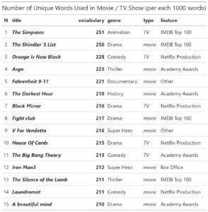
Movies_final_GT <- Movies_final %>% select (title, vocabulary, genre, type, feature) %>%
  top_n (20, vocabulary) %>% mutate (N = seq (20))
Movies_final_GT <- Movies_final_GT [,c(6,1,2,3,4,5)] %>% gt() %>%
  tab_header(
  title = "Number of Unique Words Used in Movie / TV Show (per each 1000 words)")
Using gt package we put top 15 movies by number of unique words in table. This time with header.
And we can easily save the table as graphical output.
gtsave(Movies_final_GT, filename = 'Movies_final_GT.png')
gtsave(Movies_final_GT, filename = 'Movies_final_GT.pdf')
Let`s format the table a bit.
Movies_final_GTT <- Movies_final_GT %>%
    tab_style(
    style = list(
      cell_text(weight = "bold")),
    locations = cells_column_labels(
      columns = vars(N, title, vocabulary, genre, type, feature))) %>%
  tab_style(
  style = list(
      cell_text(weight = "bold")),
locations = cells_body(
  columns = vars(title, vocabulary))) %>%
  tab_style(
    style = list(
      cell_text(style = "italic")),
locations = cells_body(
        columns = vars(title, type)))
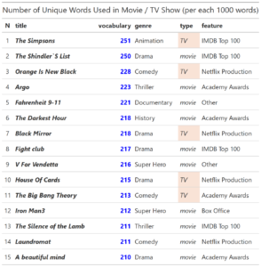
We can change cells and text colors and even make it conditional (for instance, only ‘type == TV’).
Movies_final_GTT <- Movies_final_GTT %>%
  tab_style(
    style = list(
      cell_text(color = "blue")),
locations = cells_body(
      columns = vars(vocabulary))) %>%
  tab_style(
    style = list(
      cell_fill(color = "#F9E3D6")),
locations = cells_body(
      columns = vars(type),
      rows = type == "TV"))
That`s it for tables and for Part 2 of my Movies text analysis. In Part 3 I plan to use ggplot2 to visualize and compare how wide vocabulary is within iconic movies, different genres, Movies vs TV Shows, IMDB TOP 100 vs Box Office All Time Best etc. See ya.
RXSpreadsheet: a new library for editing spreadsheets with Shiny
The goal of RXSpreadsheet is to create a wrapper for the x-spreadsheet JS library: https://github.com/myliang/x-spreadsheet. The x-spreadsheet JavaScript library is created by https://github.com/myliang and all credit goes to this person. RXSpreadsheet is a lightweight wrapper that allows you to use this library in your Shiny applications (without any JavaScript knowledge).
The editor has most common spreadsheet functionalities such as styling, validation and functions.
 You can test RXSpreadsheet by installing the GitHub version with devtools::install_github(‘MichaelHogers/RXSpreadsheet’) and subsequently running RXSpreadsheet::runExample().
This wrapper was made by Jiawei Xu and Michael Hogers. We are aiming for a CRAN release over the coming weeks. Special thanks to NPL Markets for encouraging us to release open source software.
You can test RXSpreadsheet by installing the GitHub version with devtools::install_github(‘MichaelHogers/RXSpreadsheet’) and subsequently running RXSpreadsheet::runExample().
This wrapper was made by Jiawei Xu and Michael Hogers. We are aiming for a CRAN release over the coming weeks. Special thanks to NPL Markets for encouraging us to release open source software. Hands-on: How to build an interactive map in R-Shiny: An example for the COVID-19 Dashboard
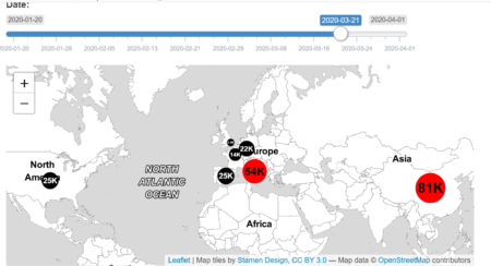
It has been two years since I started to develop various interactive web applications by using R-Shiny packages. Due to Coronavirus disease (COVID-19) at this moment, I spent some time at home on preparing a simple COVID-19 related Dashboard. To share my experiences and consideration, especially those about how to create interactive maps, the following details has been discussed.
Data Source
Dataset (data/key-countries-pivoted.csv) from Github (https://github.com/datasets/covid-19), which contains the data of daily confirmed cases of COVID-19 since 22th Jan 2020 from the eight most rapidly-spread countries (China, USA, United Kingdom, Italy, France, Germany, Spain and Iran), has been used. An example of overview of the dataset is given as follows:
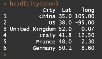
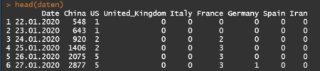 In addition, the geographic coordinates (Latitude and Longitude) of the centroids of these countries have been collected for placing charts in the leaflet map.
R Shiny: Introduction
Shiny application consists of two components, a user interface object and a server function. In user interface object, you are able to create dynamic dashboard interface, while the server function contains code provides an interactive connection between objects used for input and output. The UI object and server function will be further listed, respectively.
R library
We use the R library leaflet, which is a Javascript Library and allows users to create and customize interactive maps. For more details, we refer users to the link: https://cran.r-project.org/web/packages/leaflet/index.html
 library(shiny)
 library(leaflet.minicharts)
 library(leaflet)
Shiny-UI
The user Interface is constructed as follows, where two blocks are included. The upper block shows the worldwide COVID-19 distribution and the total number of the confirmed cases of each country. The amount of cases is labelled separately and those countries with more than 500,000 cases are marked as red, otherwise black. Note that the function leafletOutput() is used for turning leaflet map object into an interface output.
 In the lower block, we are able to visualize the time dependent development of confirmed cases for a selected country and time history. The classical layout sideBarLayout, which consists of a sidebar (sidebarPanel()) and the main area (mainPanel()), is used. Moreover, a checkbox is provided to select whether plotting the daily new confirmed cases is desired.
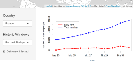
The R code for UI is given as follows:
 ui<- fluidPage(
   #Assign Dasbhoard title
   titlePanel("COVID19 Analytics"),

  # Start:  the First Block
  # Sliderinput: select from the date between 01.20.2020
  # and 01.04.2020
  sliderInput(inputId = "date", "Date:", min =
  as.Date("2020-01-20"), max = as.Date("2020-04-01"),
  value = as.Date("2020-03-01"), width = "600px"),

  # plot leaflet object (map)
  leafletOutput(outputId = "distPlot", width = "700px",
  height = "300px"),
  #End:  the First Block

  #Start: the second Block
  sidebarLayout(

    #Sidebar Panel: the selected country, history and
    #whether to plot daily new confirmed cases.
    sidebarPanel(
      selectInput("selectedcountry", h4("Country"), choices
      =list("China","US","United_Kingdom","Italy","France",
      "Germany", "Spain"), selected = "US"),
      selectInput("selectedhistoricwindow", h4("History"),
      choices = list("the past 10 days", "the past 20
      days"), selected = "the past 10 days"),
      checkboxInput("dailynew", "Daily new infected",
      value = TRUE),
      width = 3
    ),

    #Main Panel: plot the selected values
    mainPanel (
      plotOutput(outputId = "Plotcountry", width = "500px",
      height = "300px")
    )
  ),
  #End: the second Block
)
Shiny-ServerInput and output objects are connected in the Server function. Note that, the input arguments are stored in a list-like object and each input argument is identified under its unique name, for example the sliderInput is named after “date”.
server <- function(input, output){

  #Assign output$distPlot with renderLeaflet object
  output$distPlot <- renderLeaflet({

    # row index of the selected date (from input$date)
    rowindex = which(as.Date(as.character(daten$Date),
    "%d.%m.%Y") ==input$date)

    # initialise the leaflet object
    basemap= leaflet()  %>%
      addProviderTiles(providers$Stamen.TonerLite,
      options = providerTileOptions(noWrap = TRUE))

    # assign the chart colors for each country, where those
    # countries with more than 500,000 cases are marked
    # as red, otherwise black
    chartcolors = rep("black",7)
    stresscountries
    = which(as.numeric(daten[rowindex,c(2:8)])>50000)
    chartcolors[stresscountries]
    = rep("red", length(stresscountries))

    # add chart for each country according to the number of
    # confirmed cases to selected date
    # and the above assigned colors
    basemap %>%
      addMinicharts(
        citydaten$long, citydaten$Lat,
        chartdata = as.numeric(daten[rowindex,c(2:8)]),
        showLabels = TRUE,
        fillColor = chartcolors,
        labelMinSize = 5,
        width = 45,
        transitionTime = 1
      )
  })

  #Assign output$Plotcountry with renderPlot object
  output$Plotcountry <- renderPlot({

    #the selected country
    chosencountry = input$selectedcountry

    #assign actual date
    today = as.Date("2020/04/02")

    #size of the selected historic window
    chosenwindow = input$selectedhistoricwindow
    if (chosenwindow == "the past 10 days")
       {pastdays = 10}
    if (chosenwindow  == "the past 20 days")
       {pastdays = 20}

    #assign the dates of the selected historic window
    startday = today-pastdays-1
    daten$Date=as.Date(as.character(daten$Date),"%d.%m.%Y")
    selecteddata
    = daten[(daten$Date>startday)&(daten$Date<(today+1)),
    c("Date",chosencountry)]

    #assign the upperbound of the y-aches (maximum+100)
    upperboundylim = max(selecteddata[,2])+100

    #the case if the daily new confirmed cases are also
    #plotted
    if (input$dailynew == TRUE){

      plot(selecteddata$Date, selecteddata[,2], type = "b",
      col = "blue", xlab = "Date",
      ylab = "number of infected people", lwd = 3,
      ylim = c(0, upperboundylim))
      par(new = TRUE)
      plot(selecteddata$Date, c(0, diff(selecteddata[,2])),
      type = "b", col = "red", xlab = "", ylab =
      "", lwd = 3,ylim = c(0,upperboundylim))

      #add legend
      legend(selecteddata$Date[1], upperboundylim*0.95,
      legend=c("Daily new", "Total number"),
      col=c("red", "blue"), lty = c(1,1), cex=1)
    }

    #the case if the daily new confirmed cases are
    #not plotted
    if (input$dailynew == FALSE){

      plot(selecteddata$Date, selecteddata[,2], type = "b",
      col = "blue", xlab = "Date",
      ylab = "number of infected people", lwd = 3,
      ylim = c(0, upperboundylim))
      par(new = TRUE)

      #add legend
      legend(selecteddata$Date[1], upperboundylim*0.95,
      legend=c("Total number"), col=c("blue"),
      lty = c(1), cex=1)
    }

  })

}
Shiny-UIAt the end, we create a complelte application by using the shinyApp function.
shinyApp(ui = ui, server = server)The Dashboard is deployed under the following URL: https://sangmeng.shinyapps.io/COVID19/
Easy text loading and cleaning using readtext and textclean packages. Movies text analysis. Part 1
My primary goal was to research popular movies vocabulary – words all those heroes actually saying to us and put well known movies onto the scale from the ones with the widest lexicon down to below average range despite possible crowning by IMDB rating, Box Office revenue or number / lack of Academy Awards.
This post is the 1st Part of the Movies text analysis and covers Text loading and cleaning using readtext and textclean packages.
My first challenge was texts source – I saw text mining projects based on open data scripts but I wanted something new, more direct and, as close to what we actually hear AND read from the screen.
I decided directly save subtitles while streaming using Chrome developer panel.
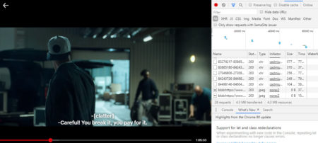
It requires further transformation through the chain .xml > .srt > .txt (not covered here).
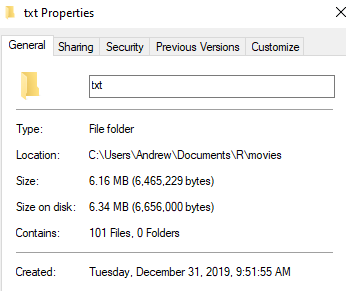
Since we have .txt files ready, let`s start from downloading of texts stored in separate folder (1movie = 1 file).
the same with () +()
Stop cut the weed, let`s replace the rest): @#$%&
In Movies text analysis. Part 2. I plan to compare how wide, in general, vocabulary is within iconic movies, different genres, Movies vs TV Shows, IMDB TOP 100 vs Box Office All Time Best etc.
In addition, having text data and the movies text length I Planned to check #of words per minute parameter to defy or confirm hypothesis that movies speech is significantly different in range and slower overall than normal speech benchmark in 120-150 WPM (words per minute).
It requires further transformation through the chain .xml > .srt > .txt (not covered here).
Since we have .txt files ready, let`s start from downloading of texts stored in separate folder (1movie = 1 file).
library(readtext)
text_raw <-readtext(paste0(path="C:/Users/Andrew/Documents/R/movies/txt/*"))
text <- gsub("\r?\n|\r", " ", text_raw)
To go further it is important to understand what is text and what is noise here. Since subtitles are real text representation of entire movie, its text part contains:
- Speech (actual text)
- Any sound (made by heroes/characters or around)
- Speakers / characters marks (who is saying)
- Intro / end themes
- Other text
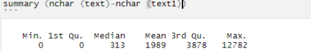
library (textclean)

text1 <- str_replace_all (text, "\\[.*?\\]", "")
text1_nchar <- sum (nchar (text1))
It is important to check how hard your trim your "garden", you could do it element-wise if the summary shows any odd losses or, in opposite, very little decrease of characters #.
the same with () +()
text2 <- str_replace_all(text1, "\\(.*?\\)", "")
text2_nchar <- sum (nchar (text2))
Do not forget any odd characters detected, like, in my case, ‘File:’
text3 <- str_replace (text2,'File:', '')
text3_nchar <- sum (nchar (text3))
Now is the trickiest part, other brackets - ♪♪ Ideally, it requires you to know the text well to distinct theme songs and background music from the situation where singing is the way the heroes “talk” to us. For instance musicals or a lot of kids movies.
text4 <- str_replace_all(text3,"\\âTª.*?\\âTª", "")
text4_nchar <- sum (nchar (text4))
Speech markers e.g. JOHN:
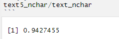
text5 <- str_replace_all(text4,"[a-zA-Z]+:", "")
text5_nchar <- sum (nchar (text5))
Check % of total cut
Stop cut the weed, let`s replace the rest): @#$%&
text6 <- replace_symbol(text5, dollar = TRUE, percent = TRUE, pound = TRUE,
                        at = TRUE, and = TRUE, with = TRUE)
text6_nchar <- sum (nchar (text6))

#time stamps
text7 <- replace_time(text6, pattern = "(2[0-3]|[01]?[0-9]):([0-5][0-9])[.:]?([0-5]?[0-9])?")
text7_nchar <- sum (nchar (text7))

#date to text
replace_date_pattern <- paste0(
  '([01]?[0-9])[/-]([0-2]?[0-9]|3[01])[/-]\\d{4}|\\d{4}[/-]',
  '([01]?[0-9])[/-]([0-2]?[0-9]|3[01])')
text8 <- replace_time(text7, pattern = replace_date_pattern)
text8_nchar <- sum (nchar (text8))

#numbers to text, e.g. 8 = eight
text9 <- replace_number(text8, num.paste = FALSE, remove = FALSE)
text9_nchar <- sum (nchar (text9))
Now texts are clean enough and ready for further analysis. That`s it for Movies text analysis. Part 1.In Movies text analysis. Part 2. I plan to compare how wide, in general, vocabulary is within iconic movies, different genres, Movies vs TV Shows, IMDB TOP 100 vs Box Office All Time Best etc.
In addition, having text data and the movies text length I Planned to check #of words per minute parameter to defy or confirm hypothesis that movies speech is significantly different in range and slower overall than normal speech benchmark in 120-150 WPM (words per minute).
“Those who can, do; those who can’t – use computer simulation.”
“Those who can, do; those who can’t – use computer simulation.” This quote was inspired by playwright George Bernard Shaw. Computer simulation is a powerful tool that attempts to reproduce the behavior of some real-world system by sampling from one or more probability distributions. It can help explain and illustrate difficult concepts such as the Monty Hall game show problem. It can also solve problems that are hard or impossible to solve directly.
One example of a problem of this latter type is the probability distribution of the sum of n independent random variables each having probability distribution g, where n is also a random variable having probability distribution f. This is a special case of a statistical subject called convolutions, where one calculates the convolution of all possible values of the individual distributions. For certain choices of f and g, such as Poisson for f and gamma for g, the resulting convolution is an integrateable function and there is no need for simulation. But for many choices of f and g, simulation or some other numerical method is needed.
A real-world use of this type of simulation is in modeling loss events of a business entity such as a bank or insurance company. The entity will have some random number of events n per year of random sizes that is modeled by a frequency distribution f such as Poisson or negative binomial. A number n is randomly selected from the frequency distribution. Then n random numbers are randomly selected from a severity distribution g such as lognormal or gamma to simulate the sizes of the n loss events. The n loss amounts are added to produce a total value of losses for one year. The process is repeated some large number of times, say 10,000, and the 10,000 numbers are ranked. If the entity is interested in the 99.9th percentile such loss, that value is the 9,990th largest value.
Base R provides functions to simulate from many probability distributions. For example, rpois(n, lamda) produces n Poisson distributed samples from a distribution having population mean lambda. Poisson is a single parameter distribution with variance equal to the mean. An alternative frequency distribution with a more flexible option for the variance is the negative binomial distribution. Its R function is rnbinom(n, mu, size) which produces n negative binomial distributed samples from a distribution having population mean mu and dispersion parameter size, where size = mu^2 / (variance – mu).
Most severity distributions are not symmetrical but rather are positively skewed with low mean and long positive tail. A random variable is lognormally distributed if the logarithm of the random variable is normally distributed. Its R function is rlnorm(n, meanlog, sdlog) which produces n lognormally distributed samples from a distribution having population mean m and standard deviation s, and here meanlog = LN(m) – .5*LN((s/m)^2 + 1)) and sdlog = .5*LN((s/m)^2+1)).
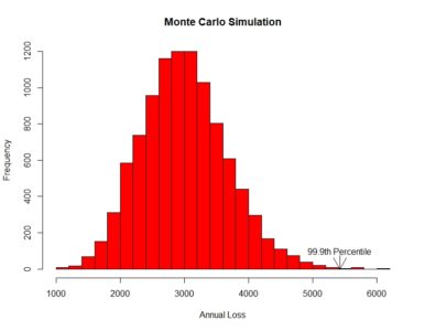
It is helpful to plot the resulting histogram of the 10,000 simulations. The real-world purpose of the exercise may be to identify the 99.9th percentile value. The R quantile function quantile(x, probs) returns the percentile value equal to probs. To display the percentile value on a plot, use the text and arrow functions. R has a text function that adds text a plot, text(x, y, label), which adds a label at coordinate (x,y). Further, R has an arrows function, arrows(x0, y0, x1, y1, code=2), which draws an arrow from (x0, y0) to (x1, y1) with code 2 drawing the arrowhead at (x1, y1).
The following is the R code and resulting histogram plot of a negative binomial frequency and lognormal severity simulation. The user input values are based on the mean and standard deviation values of a dataset.
# Monte Carlo simulation. Negative binomial frequency, lognormal severity.
# negbinom
nb_m <- 50 # This is a user input.
nb_sd <- 10 # This is a user input.
nb_var <- nb_sd^2
nb_size <- nb_m^2/(nb_var – nb_m)
# lognorm
xbar <- 60 # This is a user input.
sd <- 40 # This is a user input.
l_mean <- log(xbar) – .5*log((sd/xbar)^2 + 1)
l_sd <- sqrt(log((sd/xbar)^2 + 1))
num_sims <- 10000 # This is a user input.
set.seed(1234) # This is a user input.
rtotal <- vector()
for (i in 1:num_sims)
{
nb_random <- rnbinom(n=1, mu=nb_m, size=nb_size)
l_random <- rlnorm(nb_random, meanlog=l_mean, sdlog=l_sd)
rtotal[i] <- sum(l_random)
}
rtotal <- sort(rtotal)
m <- round(mean(rtotal), digits=0)
percentile_999 <- round(quantile(rtotal, probs=.999), digits=0)
print(paste(“Mean = “, m, ” 99.9th percentile = “, percentile_999))
hist(rtotal, breaks=20, col=”red”, xlab=”Annual Loss”, ylab=”Frequency”,
main=”Monte Carlo Simulation”)
text(percentile_999, 100, “99.9th Percentile”)
arrows(percentile_999,75, percentile_999,0, code=2)
 [contact-form][contact-field label=”Name” type=”name” required=”true” /][contact-field label=”Email” type=”email” required=”true” /][contact-field label=”Website” type=”url” /][contact-field label=”Message” type=”textarea” /][/contact-form]
A real-world use of this type of simulation is in modeling loss events of a business entity such as a bank or insurance company. The entity will have some random number of events n per year of random sizes that is modeled by a frequency distribution f such as Poisson or negative binomial. A number n is randomly selected from the frequency distribution. Then n random numbers are randomly selected from a severity distribution g such as lognormal or gamma to simulate the sizes of the n loss events. The n loss amounts are added to produce a total value of losses for one year. The process is repeated some large number of times, say 10,000, and the 10,000 numbers are ranked. If the entity is interested in the 99.9th percentile such loss, that value is the 9,990th largest value.
Base R provides functions to simulate from many probability distributions. For example, rpois(n, lamda) produces n Poisson distributed samples from a distribution having population mean lambda. Poisson is a single parameter distribution with variance equal to the mean. An alternative frequency distribution with a more flexible option for the variance is the negative binomial distribution. Its R function is rnbinom(n, mu, size) which produces n negative binomial distributed samples from a distribution having population mean mu and dispersion parameter size, where size = mu^2 / (variance – mu).
Most severity distributions are not symmetrical but rather are positively skewed with low mean and long positive tail. A random variable is lognormally distributed if the logarithm of the random variable is normally distributed. Its R function is rlnorm(n, meanlog, sdlog) which produces n lognormally distributed samples from a distribution having population mean m and standard deviation s, and here meanlog = LN(m) – .5*LN((s/m)^2 + 1)) and sdlog = .5*LN((s/m)^2+1)).
It is helpful to plot the resulting histogram of the 10,000 simulations. The real-world purpose of the exercise may be to identify the 99.9th percentile value. The R quantile function quantile(x, probs) returns the percentile value equal to probs. To display the percentile value on a plot, use the text and arrow functions. R has a text function that adds text a plot, text(x, y, label), which adds a label at coordinate (x,y). Further, R has an arrows function, arrows(x0, y0, x1, y1, code=2), which draws an arrow from (x0, y0) to (x1, y1) with code 2 drawing the arrowhead at (x1, y1).
The following is the R code and resulting histogram plot of a negative binomial frequency and lognormal severity simulation. The user input values are based on the mean and standard deviation values of a dataset.
# Monte Carlo simulation. Negative binomial frequency, lognormal severity.
# negbinom
nb_m <- 50 # This is a user input.
nb_sd <- 10 # This is a user input.
nb_var <- nb_sd^2
nb_size <- nb_m^2/(nb_var – nb_m)
# lognorm
xbar <- 60 # This is a user input.
sd <- 40 # This is a user input.
l_mean <- log(xbar) – .5*log((sd/xbar)^2 + 1)
l_sd <- sqrt(log((sd/xbar)^2 + 1))
num_sims <- 10000 # This is a user input.
set.seed(1234) # This is a user input.
rtotal <- vector()
for (i in 1:num_sims)
{
nb_random <- rnbinom(n=1, mu=nb_m, size=nb_size)
l_random <- rlnorm(nb_random, meanlog=l_mean, sdlog=l_sd)
rtotal[i] <- sum(l_random)
}
rtotal <- sort(rtotal)
m <- round(mean(rtotal), digits=0)
percentile_999 <- round(quantile(rtotal, probs=.999), digits=0)
print(paste(“Mean = “, m, ” 99.9th percentile = “, percentile_999))
hist(rtotal, breaks=20, col=”red”, xlab=”Annual Loss”, ylab=”Frequency”,
main=”Monte Carlo Simulation”)
text(percentile_999, 100, “99.9th Percentile”)
arrows(percentile_999,75, percentile_999,0, code=2)
[contact-form][contact-field label=”Name” type=”name” required=”true” /][contact-field label=”Email” type=”email” required=”true” /][contact-field label=”Website” type=”url” /][contact-field label=”Message” type=”textarea” /][/contact-form]