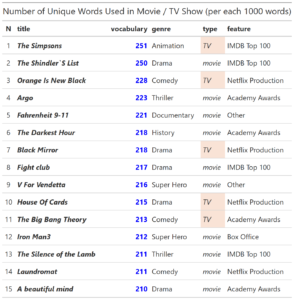
This time I am sharing analysis of the most popular movies / TV shows across Netflix, Disney+, Hulu and HBOmax on weekly basis, instead of daily, with anticipation of better trends catching.
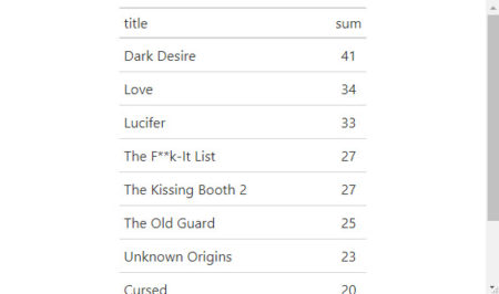
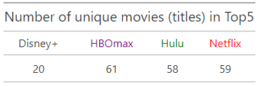
So, let`s count how many movies made the top5, I assume it is less than 5 *60…
library(tidyverse)
library (gt)

platforms <- c('Disney+','HBOmax', 'Hulu', 'Netflix') # additionally, load CSV data using readr
Wrangle raw data – reverse (fresh date first), take top 5, take last 60 days
fjune_dt % rev () %>% slice (1:5) %>% select (1:60)
fdjune_dt % rev () %>% slice (1:5) %>% select (1:60)
hdjune_dt % rev () %>% slice (1:5) %>% select (1:60)
hulu_dt % rev () %>% slice (1:5) %>% select (1:60)
Gather it together and count the number of unique titles in Top5 for 60 days
fjune_dt_gathered <- gather (fjune_dt)
fdjune_dt_gathered <- gather (fdjune_dt)
hdjune_dt_gathered <- gather (hdjune_dt)
hulu_dt_gathered <- gather (hulu_dt)
unique_fjune_gathered % length ()
unique_fdjune_gathered % length ()
unique_hdjune_gathered % length ()
unique_hulu_gathered % length ()
unique_gathered <- c(unique_fdjune_gathered, unique_hdjune_gathered, unique_hulu_gathered, unique_fjune_gathered)
unique_gathered <- as.data.frame (t(unique_gathered), stringsAsFactors = F)
colnames (unique_gathered) <- platforms
Let`s make a nice table for the results
unique_gathered_gt %
tab_header(
  title = "Number of unique movies (titles) in Top5")%>%
  tab_style(
    style = list(
      cell_text(color = "purple")),
    locations = cells_column_labels(
      columns = vars(HBOmax)))%>%
  tab_style(
    style = list(
      cell_text(color = "green")),
    locations = cells_column_labels(
      columns = vars(Hulu))) %>%
  tab_style(
    style = list(
      cell_text(color = "red")),
    locations = cells_column_labels(
      columns = vars(Netflix)))
unique_gathered_gt
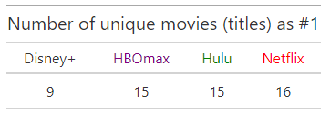
Using similar code we can count the number of unique titles which were #1 one or more days
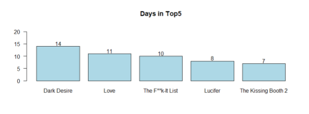
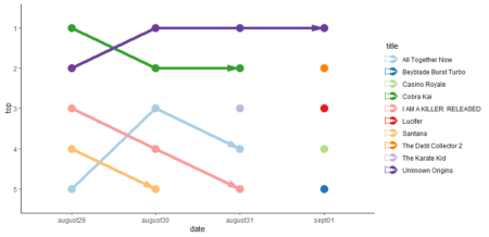
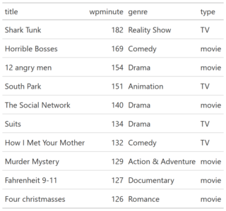
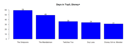
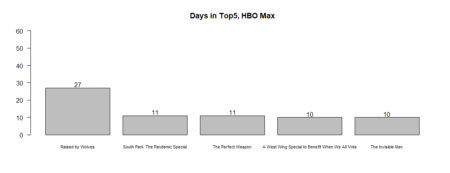
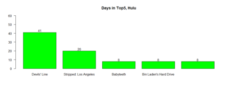
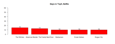
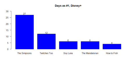
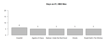
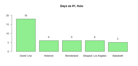
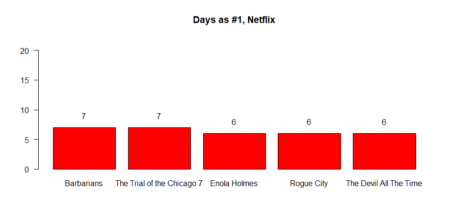
What movie was the longest in Tops / #1?
table_fjune_top5 <- sort (table (fjune_dt_gathered$value), decreasing = T) # Top5
table_fdjune_top5 <- sort (table (fdjune_dt_gathered$value), decreasing = T)
table_hdjune_top5 <- sort (table (hdjune_dt_gathered$value), decreasing = T)
table_hulu_top5 <- sort (table (hulu_dt_gathered$value), decreasing = T)
Plotting the results
bb5fdjune <- barplot (table_fdjune_top5 [1:5], ylim=c(0,62), main = "Days in Top5, Disney+", las = 1, col = 'blue')
text(bb5fdjune,table_fdjune_top5 [1:5] +2,labels=as.character(table_fdjune_top5 [1:5]))
bb5hdjune <- barplot (table_hdjune_top5 [1:5], ylim=c(0,60), main = "Days in Top5, HBO Max", las = 1, col = 'grey', cex.names=0.7)
text(bb5hdjune,table_hdjune_top5 [1:5] +2,labels=as.character(table_hdjune_top5 [1:5]))
bb5hulu <- barplot (table_hulu_top5 [1:5], ylim=c(0,60), main = "Days in Top5, Hulu", las = 1, col = 'green')
text(bb5hulu,table_hulu_top5 [1:5] +2,labels=as.character(table_hulu_top5 [1:5]))
bb5fjune <- barplot (table_fjune_top5 [1:5], ylim=c(0,60), main = "Days in Top5, Netflix", las = 1, col = 'red')
text(bb5fjune,table_fjune_top5 [1:5] +2,labels=as.character(table_fjune_top5 [1:5]))
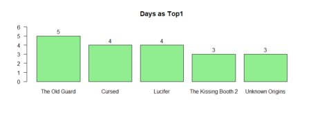
The same for the movies / TV shows reached the first place in weekly count
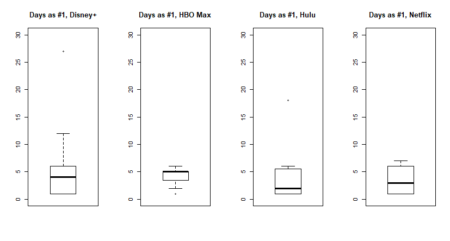
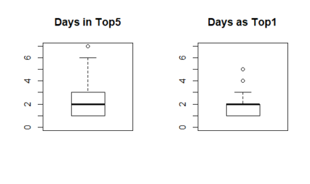
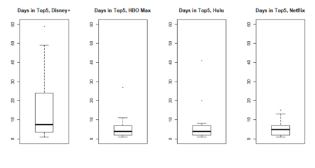
Average days in top distribution
#top 5
ad5_fjune <- as.data.frame (table_fjune_top5, stringsAsFActrors=FALSE)
ad5_fdjune <- as.data.frame (table_fdjune_top5, stringsAsFActrors=FALSE)
ad5_hdjune <- as.data.frame (table_hdjune_top5, stringsAsFActrors=FALSE)
ad5_hulu <- as.data.frame (table_hulu_top5, stringsAsFActrors=FALSE)
par (mfcol = c(1,4))
boxplot (ad5_fdjune$Freq, ylim=c(0,20), main = "Days in Top5, Disney+")
boxplot (ad5_hdjune$Freq, ylim=c(0,20), main = "Days in Top5, HBO Max")
boxplot (ad5_hulu$Freq, ylim=c(0,20), main = "Days in Top5, Hulu")
boxplot (ad5_fjune$Freq, ylim=c(0,20), main = "Days in Top5, Netflix")
The same for the movies / TV shows reached the first place in weekly count (#1)