Introduction
The rest of this post demonstrates how you can download iNaturalist observations in R using the rinat package, and then map them using leaflet. We’ll also use functions from sf and dplyr. These are very common R packages in data science, and there are lot of online resources that teach you how to use them.
Our study area will be Placerita Canyon State Park in Los Angeles County, California. If you want to jump ahead to see the final product, click here.
Import the Park Boundary
First we load the packages we’re going use:library(rinat)
library(sf)
library(dplyr)
library(tmap)
library(leaflet)
## Load the conflicted package and set preferences
library(conflicted)
conflict_prefer("filter", "dplyr", quiet = TRUE)
conflict_prefer("count", "dplyr", quiet = TRUE)
conflict_prefer("select", "dplyr", quiet = TRUE)
conflict_prefer("arrange", "dplyr", quiet = TRUE)
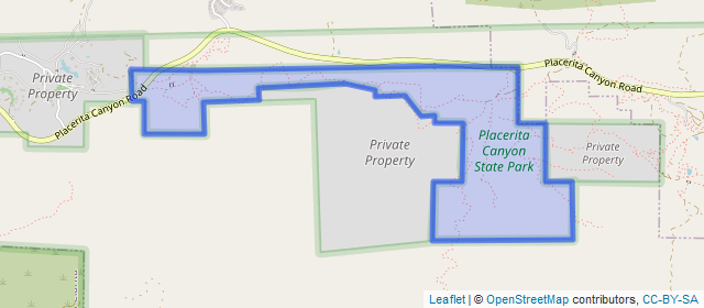
Now we can import the park boundary which is saved as a geojson file. We use the sf package to import and transform the boundary to geographic coordinates, and leaflet to plot it:
placertia_sf <- st_read("placertia_canyon_sp.geojson", quiet = TRUE) %>%
  st_transform(4326)

leaflet(placertia_sf) %>%
  addTiles() %>%
  addPolygons()
Get the Bounding Box
Next, we get the bounding box of the study area, so we can pass it to the iNaturalist API to tell it which area we’re interested in:placertia_bb <- placertia_sf %>% st_bbox() placertia_bb
##       xmin       ymin       xmax       ymax
## -118.47216   34.36698 -118.43764   34.37820
Download data
Now we are ready to retrieve iNaturalist observations. rinat makes this easy with get_inat_obs().
Downloading Etiquette
The non-profit that supports iNaturalist doesn’t charge for downloading data, because they believe in open data and supporting citizen science initiatives. They also don’t require registration for simply downloading observations. That being said, downloading data consumes resources that can affect other users, and it’s bad form (and bad programming) to download data unnecessarily.
There are a few best practices for downloading data in ways that won’t cause problems for other users:
- Use the server-side filters the API provides to only return results for your area of interest and your taxon(s) of interest. See below for examples of sending spatial areas and a taxon name when calling the API from R.
- Always save your results to disk, and don’t download data more than once. Your code should check to see if you’ve already downloaded something before getting it again.
- Don’t download more than you need. The API will throttle you (reduce your download speed) if you exceed more than 100 calls per minute. Spread it out.
- The API is not designed for bulk downloads. For that, look at the Export tool.
We’ll use the bounds argument in get_inat_obs() to specify the extent of our search. bounds takes 4 coordinates. Our study area is not a pure rectangle, but we’ll start with the bounding box and then apply an additional mask to remove observations outside the park boundary.
For starters we’ll just download the most recent 100 iNaturalist observations within the bounding box. (There are actually over 3000, but that would make for a very crowded map!). The code below first checks if the data have already been downloaded, to prevent downloading data twice.
search_results_fn <- "placertia_bb_inat.Rdata"

if (file.exists(search_results_fn)) {
  load(search_results_fn)

} else {
  # Note we have to rearrange the coordinates of the bounding box a
  # little bit to give get_inat_obs() what it expects
  inat_obs_df <- get_inat_obs(bounds = placertia_bb[c(2,1,4,3)],
                            taxon_name = NULL,
                            year = NULL,
                            month = NULL,
                            maxresults = 100)

  ## Save the data frame to disk
  save(inat_obs_df, file = search_results_fn)
}
See what we got back:
dim(inat_obs_df)
## [1] 100 36
glimpse(inat_obs_df)
## Rows: 100
## Columns: 36
## $ scientific_name                   "Sceloporus occidentalis", "Eriogonum~
## $ datetime                          "2021-09-04 14:01:55 -0700", "2021-08~
## $ description                       "", "", "", "", "", "", "", "", "", "~
## $ place_guess                       "Placerita Canyon State Park, Newhall~
## $ latitude                          34.37754, 34.37690, 34.37691, 34.3764~
## $ longitude                         -118.4571, -118.4598, -118.4597, -118~
## $ tag_list                          "", "", "", "", "", "", "", "", "", "~
## $ common_name                       "Western Fence Lizard", "California b~
## $ url                               "https://www.inaturalist.org/observat~
## $ image_url                         "https://inaturalist-open-data.s3.ama~
## $ user_login                        "bmelchiorre", "ericas3", "ericas3", ~
## $ id                                94526862, 92920757, 92920756, 9291801~
## $ species_guess                     "Western Fence Lizard", "", "", "", "~
## $ iconic_taxon_name                 "Reptilia", "Plantae", "Plantae", "Pl~
## $ taxon_id                          36204, 54999, 52854, 58014, 64121, 55~
## $ num_identification_agreements     2, 0, 0, 0, 0, 1, 0, 0, 0, 0, 1, 0, 1~
## $ num_identification_disagreements  0, 0, 0, 0, 0, 0, 0, 0, 0, 0, 0, 0, 0~
## $ observed_on_string                "Sat Sep 04 2021 14:01:55 GMT-0700 (P~
## $ observed_on                       "2021-09-04", "2021-08-29", "2021-08-~
## $ time_observed_at                  "2021-09-04 21:01:55 UTC", "2021-08-2~
## $ time_zone                         "Pacific Time (US & Canada)", "Pacifi~
## $ positional_accuracy               5, 3, 4, 4, 16, 4, 41, 41, 26, 9, NA,~
## $ public_positional_accuracy        5, 3, 4, 4, 16, 4, 41, 41, 26, 9, NA,~
## $ geoprivacy                        "", "", "", "", "", "", "", "", "", "~
## $ taxon_geoprivacy                  "open", "", "", "", "", "", "", "", "~
## $ coordinates_obscured              "false", "false", "false", "false", "~
## $ positioning_method                "", "", "", "", "", "", "", "", "", "~
## $ positioning_device                "", "", "", "", "", "", "", "", "", "~
## $ user_id                           4985856, 404893, 404893, 404893, 3214~
## $ created_at                        "2021-09-12 02:16:03 UTC", "2021-08-2~
## $ updated_at                        "2021-09-12 06:28:20 UTC", "2021-08-2~
## $ quality_grade                     "research", "needs_id", "needs_id", "~
## $ license                           "CC-BY-NC", "CC-BY-NC-SA", "CC-BY-NC-~
## $ sound_url                         NA, NA, NA, NA, NA, NA, NA, NA, NA, N~
## $ oauth_application_id              3, 333, 333, 333, 3, 3, 3, 3, 3, 3, N~
## $ captive_cultivated                "false", "false", "false", "false", "~
Next, in order to spatially filter the observations using the park boundary, we convert the data frame into a sf object. At the same time we’ll select just a few of the columns for our map:
inat_obs_sf <- inat_obs_df %>%
select(longitude, latitude, datetime, common_name,
      scientific_name, image_url, user_login) %>%
  st_as_sf(coords=c("longitude", "latitude"), crs=4326)

dim(inat_obs_sf)
## [1] 100 6Next, filter out observations that lie outside Placerita Canyon SP. How many are left?
inat_obs_pcsp_sf <- inat_obs_sf %>% st_intersection(placertia_sf)
nrow(inat_obs_pcsp_sf)
## [1] 90Next, add a column to the attribute table containing HTML code that will appear in the popup windows:
inat_obs_pcsp_popup_sf <- inat_obs_pcsp_sf %>%
  mutate(popup_html = paste0("<p><b>", common_name, "</b><br/>",
                        "<i>", scientific_name, "</i></p>",
                        "<p>Observed: ", datetime, "<br/>",
                        "User: ", user_login, "</p>",
                        "<p><img src='", image_url, "' style='width:100%;'/></p>")
)
Map the Results
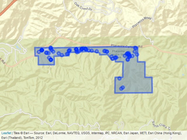
Finally, we have everything we need to map the results with leaflet. Zoom-in and click on an observation to see details about it.htmltools::p("iNaturalist Observations in Placerita Canyon SP",
htmltools::br(),
inat_obs_pcsp_popup_sf$datetime %>%
as.Date() %>%
range(na.rm = TRUE) %>%
paste(collapse = " to "),
style = "font-weight:bold; font-size:110%;")
leaflet(placertia_sf) %>%
addProviderTiles("Esri.WorldStreetMap") %>%
addPolygons() %>%
addCircleMarkers(data = inat_obs_pcsp_popup_sf,
popup = ~popup_html,
radius = 5)
iNaturalist Observations in Placerita Canyon SP
2006-01-04 to 2021-09-04
Click on the map to open in a new tab
Map the Arachnids
The iNaturalist API supports taxon searching. If you pass it the name of a genus, for example, it will restrict results to only observations from that genus. Likewise for family, order, class, etc. Observations that don’t have a scientific name assigned will be left out.You can do a taxon search from R by passing the taxon_name argument in get_inat_obs(). Below we’ll ask for the Arachnid class, which includes spiders, scorpions, ticks, and other arthropods. This code should all look familiar by now:
search_arachnid_fn <- "placertia_arachnid_obs.Rdata"
if (file.exists(search_arachnid_fn)) {
  load(search_arachnid_fn)
} else {
  inat_arachnid_df <- get_inat_obs(bounds = placertia_bb[c(2,1,4,3)],
                            taxon_name = "Arachnida",
                            year = NULL,
                            month = NULL,
                            maxresults = 100)
  save(inat_arachnid_df, file = search_arachnid_fn)
}

inat_arachnid_pcsp_popup_sf <- inat_arachnid_df %>%
  select(longitude, latitude, datetime, common_name, scientific_name, image_url, user_login) %>%
  st_as_sf(coords=c("longitude", "latitude"), crs=4326) %>%
  st_intersection(placertia_sf) %>%
  mutate(popup_html = paste0("<p><b>", common_name, "</b><br/>",
                             "<i>", scientific_name, "</i></p>",
                             "<p>Observed: ", datetime, "<br/>",
                             "User: ", user_login, "</p>",
                             "<p><img src='", image_url,
                             "' style='width:100%;'/></p>"))

htmltools::p("Arachnids in Placerita Canyon SP", style = "font-weight:bold; font-size:110%;")

leaflet(placertia_sf) %>%
  addProviderTiles("Esri.WorldStreetMap") %>%
  addPolygons() %>%
  addCircleMarkers(data = inat_arachnid_pcsp_popup_sf,
                   popup = ~popup_html,
                   radius = 5)
Arachnids in Placerita Canyon SP
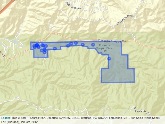
Click on the map to open in a new tab
Summary
The iNaturalist API allows you to download observations from a global community of naturalists, which is pretty powerful. This Tech Note showed you how to create a map of iNaturalist observations within a specific area and for a specific taxon using the rinat and leaflet packages for R.A couple caveats are worth noting. A limitation of this method is that the data are static. In other words, to get the latest data your have to re-query the API again. It isn’t ‘live’ like a feature service.
Also, although leaflet works well for small to medium sized datasets, you wouldn’t want to use this mapping tool for massive amounts of spatial data. With leaflet, all of the geographic information and popup content are saved in the HTML file, and rendering is done on the client. This generally makes it extremely fast because everything is in memory. But if the data overwhelm memory it can slow your browser to a crawl. If you have to map hundreds of thousands of points, for example, you would need a different approach for both downloading and visualizing the data.