Mastering Data Preprocessing in R with the `recipes` Package

Data preprocessing is a critical step in any machine learning workflow. It ensures that your data is clean, consistent, and ready for modeling. In R, the recipes package provides a powerful and flexible framework for defining and applying preprocessing steps. In this blog post, we’ll explore how to use recipes to preprocess data for machine learning, step by step.

Here’s what we’ll cover in this blog:

1. Introduction to the `recipes` Package
   - What is the `recipes` package, and why is it useful?

2. Why Preprocess Data?
   - The importance of centering, scaling, and encoding in machine learning.

3. Step-by-Step Preprocessing with `recipes`  
   - How to create a preprocessing recipe.  
   - Centering and scaling numeric variables.  
   - One-hot encoding categorical variables.

4. Applying the Recipe  
   - How to prepare and apply the recipe to training and testing datasets.

5. Example: Preprocessing in Action  
   - A practical example of preprocessing a dataset.

6. Why Use `recipes`?  
   - The advantages of using the `recipes` package for preprocessing.

7. Conclusion  
   - A summary of the key takeaways and next steps.

What is the recipes Package?

The recipes package is part of the tidymodels ecosystem in R. It allows you to define a series of preprocessing steps (like centering, scaling, and encoding) in a clean and reproducible way. These steps are encapsulated in a “recipe,” which can then be applied to your training and testing datasets.


Why Preprocess Data?

Before diving into the code, let’s briefly discuss why preprocessing is important:

  1. Centering and Scaling:

    • Many machine learning algorithms (e.g., SVM, KNN, neural networks) are sensitive to the scale of features. If features have vastly different scales, the model might give undue importance to features with larger magnitudes.

    • Centering and scaling ensure that all features are on a comparable scale, improving model performance and convergence.

  2. One-Hot Encoding:

    • Machine learning algorithms typically require numeric input. Categorical variables need to be converted into numeric form.

    • One-hot encoding converts each category into a binary vector, preventing the model from assuming an ordinal relationship between categories.


Step-by-Step Preprocessing with recipes

Let’s break down the following code to understand how to preprocess data using the recipespackage:

preprocess_recipe <- recipe(target_variable ~ ., data = training_data) %>%
  step_center(all_numeric(), -all_outcomes()) %>%
  step_scale(all_numeric(), -all_outcomes()) %>%
  step_dummy(all_nominal(), -all_outcomes(), one_hot = TRUE)

1. Creating the Recipe Object

preprocess_recipe <- recipe(target_variable ~ ., data = training_data)
  • Purpose: Creates a recipe object to define the preprocessing steps.

  • target_variable ~ .: Specifies that target_variable is the target (dependent) variable, and all other variables in training_data are features (independent variables).

  • data = training_data: Specifies the training dataset to be used.


2. Centering Numeric Variables

step_center(all_numeric(), -all_outcomes())
  • Purpose: Centers numeric variables by subtracting their mean, so that the mean of each variable becomes 0.

  • all_numeric(): Selects all numeric variables.

  • -all_outcomes(): Excludes the target variable (target_variable), as it does not need to be centered.


3. Scaling Numeric Variables

step_scale(all_numeric(), -all_outcomes())
  • Purpose: Scales numeric variables by dividing them by their standard deviation, so that the standard deviation of each variable becomes 1.

  • all_numeric(): Selects all numeric variables.

  • -all_outcomes(): Excludes the target variable (target_variable), as it does not need to be scaled.


4. One-Hot Encoding for Categorical Variables

step_dummy(all_nominal(), -all_outcomes(), one_hot = TRUE)
  • Purpose: Converts categorical variables into binary (0/1) variables using one-hot encoding.

  • all_nominal(): Selects all nominal (categorical) variables.

  • -all_outcomes(): Excludes the target variable (target_variable), as it does not need to be encoded.

  • one_hot = TRUE: Specifies that one-hot encoding should be used.


Applying the Recipe

Once the recipe is defined, you can apply it to your data:

# Prepare the recipe with the training data
prepared_recipe <- prep(preprocess_recipe, training = training_data, verbose = TRUE)

# Apply the recipe to the training data
train_data_preprocessed <- juice(prepared_recipe)

# Apply the recipe to the testing data
test_data_preprocessed <- bake(prepared_recipe, new_data = testing_data)
  • prep(): Computes the necessary statistics (e.g., means, standard deviations) from the training data to apply the preprocessing steps.

  • juice(): Applies the recipe to the training data.

  • bake(): Applies the recipe to new data (e.g., the testing set).


Example: Preprocessing in Action

Suppose the training_data dataset looks like this:

target_variable feature_1 feature_2 category
150 25 50000 A
160 30 60000 B
140 22 45000 B

Preprocessed Data

  1. Centering and Scaling:

    • feature_1 and feature_2 are centered and scaled.

  2. One-Hot Encoding:

    • category is converted into binary variables: category_A and category_B.

The preprocessed data might look like this:

target_variable feature_1_scaled feature_2_scaled category_A category_B
150 -0.5 0.2 1 0
160 0.5 0.8 0 1
140 -1.0 -0.5 0 1

Why Use recipes?

The recipes package offers several advantages:

  1. Reproducibility: Preprocessing steps are clearly defined and can be reused.

  2. Consistency: The same preprocessing steps are applied to both training and testing datasets.

  3. Flexibility: You can easily add or modify steps in the preprocessing pipeline.


Conclusion

Data preprocessing is a crucial step in preparing your data for machine learning. With the recipespackage in R, you can define and apply preprocessing steps in a clean, reproducible, and efficient way. By centering, scaling, and encoding your data, you ensure that your machine learning models perform at their best.

Ready to try it out? Install the recipes package and start preprocessing your data today!

install.packages("recipes")
library(recipes)

Happy coding! 😊
REDCapDM: a package to access and manage REDCap data

Garcia-Lerma E, Carmezim J, Satorra P, Peñafiel J, Pallares N, Santos N, Tebé C.
Biostatistics Unit, Bellvitge Biomedical Research Institute (IDIBELL)

The REDCapDM package allows users to read data exported directly from REDCap or via an API connection. It also allows users to process the previously downloaded data, create reports of queries and track the identified issues.

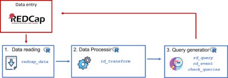
The diagram below shows the data management cycle: from data entry in REDCap to obtain data ready for the analysis.


The package structure can be divided into three main components: reading raw data, processing data and identifying queries. Typically, after collecting data in REDCap, we will have to follow these three components in order to have a final validated dataset for analysis. We will provide a user guide on how to perform each one of these steps using the package’s functions. For data processing and query identification, we will use the COVICAN data as an example (see the package vignette for more information about this built-in dataset).

Read data: redcap_data

The redcap_data function allows users to easily import data from a REDCap project into R for analysis.

To read exported data from REDCap, use the arguments data_path and dic_path to, respectively, describe the path of the R file and the REDCap project’s dictionary:

dataset <- redcap_data(data_path="C:/Users/username/example.r",
                       dic_path="C:/Users/username/example_dictionary.csv")

Note: The R and CSV files exported from REDCap must be located in the same directory.

If the REDCap project is longitudinal (contains more than one event) then a third element should be specified with the correspondence of each event with each form of the project. This csv file can be downloaded in the REDCap of the project following these steps: Project Setup < Designate Instruments for My Events < Download instrument-event mappings (CSV).

dataset <- redcap_data(data_path="C:/Users/username/example.r",
                       dic_path="C:/Users/username/example_dictionary.csv",
                       event_path="C:/Users/username/events.csv")

Note: if the project is longitudinal and the event-form file is not provided using the event_path argument, some steps of the processment can not be performed.

Another way to read data exported from a REDCap project is using an API connection. To do this, we can use the arguments uri and token which respectively refer to the uniform resource identifier of the REDCap project and the user-specific string that serves as the password:

dataset_api <- redcap_data(uri ="https://redcap.idibell.cat/api/",
                           token = "55E5C3D1E83213ADA2182A4BFDEA")

In this case, there is no need to specify the event-form file since the function will download it automatically using the API connection, if the project is longitudinal.

Remember that the token would give anyone access to all the project’s information. You should be careful about who you give this information to.

This function returns a list with 3 elements (imported data, dictionary and event-form mapping) which can then be used for further analysis or visualization.

Data process: rd_transform

The main function involved in the processing of the data is rd_transform. This function is used to process the REDCap data read into R using the redcap_data, as described above. Using the arguments of the function we can perform different type of transformations of our data.

As previously stated, we will use the built-in dataset covican as an example.

The only necessary elements that must be provided are the dataset to be transformed and the corresponding dictionary. If the project is longitudinal, as in the case of covican, also the event-form dataset should be specified. These elements can be specified directly using the output of the redcap_data function or separately in different arguments.

#Option A: list object 
covican_transformed <- rd_transform(covican)

#Option B: separately with different arguments
covican_transformed <- rd_transform(data = covican$data, 
                                    dic = covican$dictionary, 
                                    event_form = covican$event_form)

#Print the results of the transformation
covican_transformed$results
1. Recalculating calculated fields and saving them as '[field_name]_recalc'

| Total calculated fields | Non-transcribed fields | Recalculated different fields |
|:-----------------:|:----------------:|:-----------------------:|
|         2         |      0 (0%)      |         1 (50%)         |


|     field_name      | Transcribed? | Is equal? |
|:-------------------:|:------------:|:---------:|
|         age         |     Yes      |   FALSE   |
| screening_fail_crit |     Yes      |   TRUE    |

2. Transforming checkboxes: changing their values to No/Yes and changing their names to the names of its options. For checkboxes that have a branching logic, when the logic is missing their values will be set to missing

Table: Checkbox variables advisable to be reviewed

| Variables without any branching logic |
|:-------------------------------------:|
|        type_underlying_disease        |

3. Replacing original variables for their factor version

4. Deleting variables that contain some patterns

This function will return a list with the transformed dataset, dictionary and the output of the results of the transformation.

As we can see, there are 4 steps in the transformation and they are briefly explained in the output of the function. This four steps are:

        1. Recalculation of REDCap calculated fields

        2. Checkbox transformation

        3. Replacement of the original variable by its factor version

        4. Elimination of variables containing some pattern

In addition, we can change the final structure of the transformed dataset by specifying in the final_format argument whether we want our data to be split by event or by form.

For more examples and information on extra arguments, see the vignette.

Queries

Queries are very important to ensure the accuracy and reliability of a REDCap dataset. The collected data may contain missing values, inconsistencies, or other potential errors that need to be identified in order to correct them later.

For all the following examples we will use the raw transformed data: covican_transformed.

rd_query

The rd_query function allows users to generate queries by using a specific expression. It can be used to identify missing values, values that fall outside the lower and upper limit of a variable and other types of inconsistencies.

Missings

If we want to identify missing values in the variables copd and age in the raw transformed data, a list of required arguments needs to be supplied.

example <- rd_query(covican_transformed,
                    variables = c("copd", "age"),
                    expression = c("%in%NA", "%in%NA"),
                    event = "baseline_visit_arm_1")

# Printing results
example$results
Report of queries
Variables Description Event Query Total
copd Chronic obstructive pulmonary disease Baseline visit The value should not be missing 6
age Age Baseline visit The value should not be missing 5

Expressions

The rd_query function is also able to identify outliers or observations that fulfill a specific condition.

example <- rd_query(variables="age",
                    expression=">70",
                    event="baseline_visit_arm_1",
                    dic=covican_transformed$dictionary,
                    data=covican_transformed$data)

# Printing results
example$results
Report of queries
Variables Description Event Query Total
age Age Baseline visit The value should not be >70 76

More examples of both functions can be seen at the vignette.

Output

When the rd_query function is executed, it returns a list that includes a data frame with all the queries identified and a second element with a summary of the number of generated queries in each specified variable for each expression applied:

Identifier DAG Event Instrument Field Repetition Description Query Code
100-58 Hospital 11 Baseline visit Comorbidities copd · Chronic obstructive pulmonary disease The value is NA and it should not be missing 100-58-1
Report of queries
Variables Description Event Query Total
copd Chronic obstructive pulmonary disease Baseline visit The value should not be missing 6

The data frame is designed to aid users in locating each query in their REDCap project. It includes information such as the record identifier, the Data Access Group (DAG), the event in which each query can be found, along with the name and the description of the analyzed variable and a brief description of the query.

check_queries

Once the process of identifying queries is complete, the typical approach would be to adress them by modifying the original dataset in REDCap and re-run the query identification process generating a new query dataset.

The check_queries function compares the previous query dataset with the new one by using the arguments old and new, respectively. The output remains a list with 2 items, but the data frame containing the information for each query will now have an additional column (“Modification”) indicating which queries are new, which have been modified, which have been corrected, and which remain pending. Besides, the summary will show the number of queries in each one of these categories:

check <- check_queries(old = example$queries, 
                       new = new_example$queries)

# Print results
check$results
Comparison report
State Total
Pending 7
Solved 3
Miscorrected 1
New 1

There are 7 pending queries, 3 solved queries, 1 miscorrected query, and 1 new query between the previous and the new query dataset.

Note: The “Miscorrected” category includes queries that belong to the same combination of record identifier and variable in both the old and new reports, but with a different reason. For instance, if a variable had a missing value in the old report, but in the new report shows a value outside the established range, it would be classified as “Miscorrected”.

Query control output:

Identifier DAG Event Instrument Field Repetition Description Query Code Modification
100-58 Hospital 11 Baseline visit Comorbidities copd · Chronic obstructive pulmonary disease The value is NA and it should not be missing 100-58-1 Pending
100-79 Hospital 11 Baseline visit Comorbidities copd · Chronic obstructive pulmonary disease The value is NA and it should not be missing 100-79-1 New
102-113 Hospital 24 Baseline visit Demographics age · Age The value is NA and it should not be missing 102-113-1 Pending
105-11 Hospital 5 Baseline visit Comorbidities copd · Chronic obstructive pulmonary disease The value is NA and it should not be missing 105-11-1 Pending

Future improvements

In the short term, we would like to make some improvements to the query identification and tracking process to minimise errors and cover a wide range of possible structures. We would also like to extend the scope of the data processing to cover up specific transformations of the data that may be required in some specific scenarios. As a long-term plan, we would like to complement this package with the development of a shiny application to facilitate the use of the package and make it as user-friendly as possible.


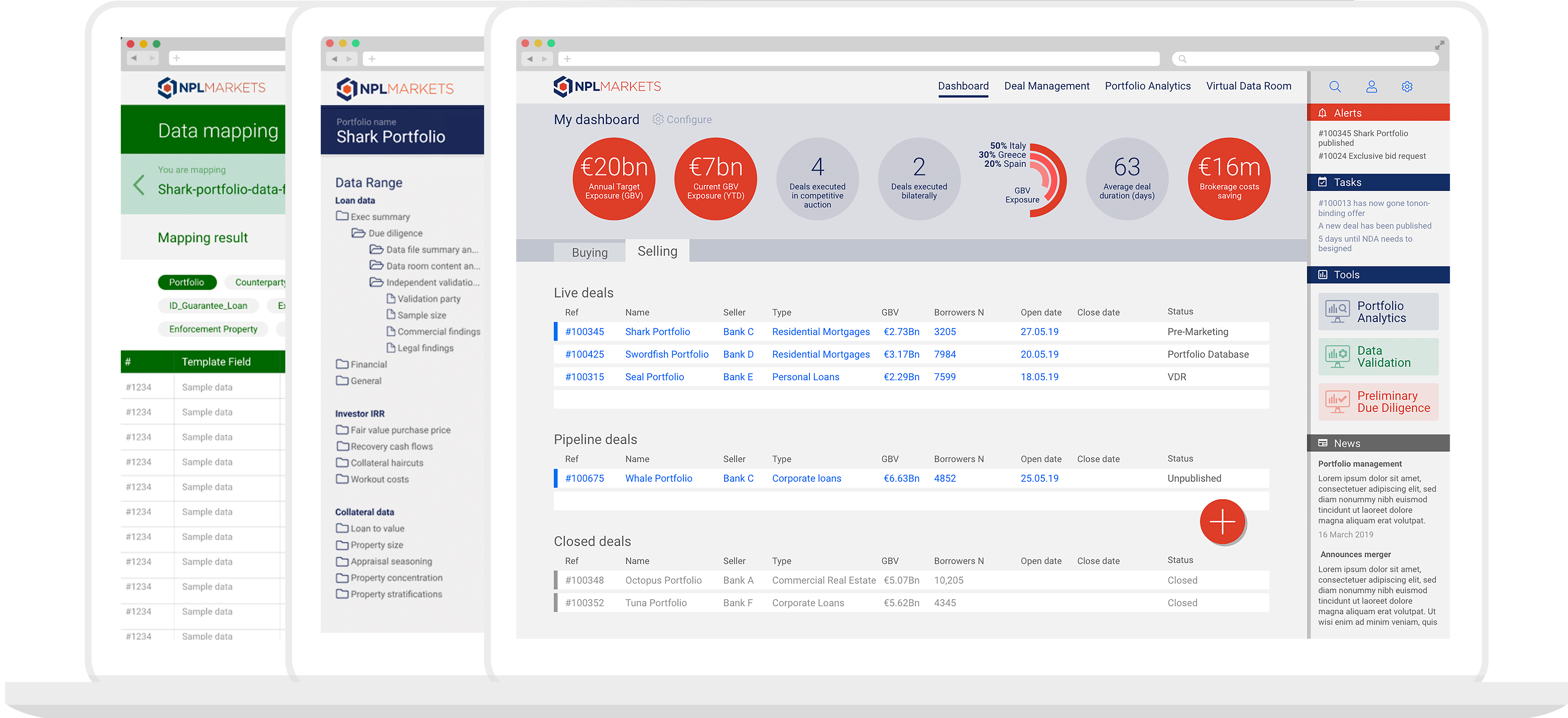
NPL Markets and R Shiny

Our mission at NPL Markets is to enable smart decision-making through innovative trading technology, advanced data analytics and a new comprehensive trading ecosystem. We focus specifically on the illiquid asset market, a market that is partially characterized by its unstructured data.

  Platform Overview


NPL Markets fully embraces R and Shiny to create an interactive platform where sellers and buyers of illiquid credit portfolios can interact with each other and use sophisticated tooling to structure and analyse credit data. 

Creating such a platform with R Shiny was a challenge, while R Shiny is extremely well suited to analyzing data, it is not entirely a generalist web framework. Perhaps it was not intended as such, but our team at NPL Markets has managed to create an extremely productive setup. 

Our development setup has a self-build ‘hot reload’ library, which we may release to a wider audience once it is sufficiently tested internally. This library allows us to update front-end and server code on the fly without restarting the entire application.

In addition to our development setup, our production environment uses robust error handling and reporting, preventing crashes that require an application to restart.

More generally, we use continuous integration and deployment and automatically create unit tests for any newly created R functions, allowing us to quickly iterate.

If you would like to know more about what we built with R and Shiny, reach out to us via our website www.nplmarkets.com