Actually, it’s both possible
This Article was originally published before on YOZM-IT as Korean
Various way of data science
There are many programming languages in the world and software that utilizes them. And those play an important role in “Data science”.
For example, if you’re using funnel analysis to improve your product, you might want to
- Compare the bounce rates of funnel stages before and after an event,
- And perform a ratio test to calculate their statistical significance.

Meanwhile, data scientists have various career backgrounds and experiences. So They tend to use the methods they’re comfortable with, including Python, R, SAS and more.
We see this quite a bit, because in most cases, the software you use at the level of business doesn’t make much of a difference.
But what happens if you “produce different results by the software used?”
The following image shows the results of running a proportion test in R, Python, and STATA with example mentioned.

You can see that even though we used the same values of 1000 and 123, the p-value, which indicates the significance of the proportion test, is slightly different for each method.
There are many reasons why the calculation value is different depending on the method used, such as
- Different algorithms in the core logic of the programming language
- Different default values of the parameters used in the function.
In the example above, if you change the value of the parameter correct in R and apply “Continuity correction” as using “correct = F” , you can see that the result is the same as in STATA.

Rounding
Next, I’ll introduce rounding for more general data analysis.

Similarly, you can see that the round changes its value depending on software.
If the fee is “0.5 billion” in some large financial transaction in business, the rounded cost could be zero or 1 billion, depending on how you calculate the rounding.
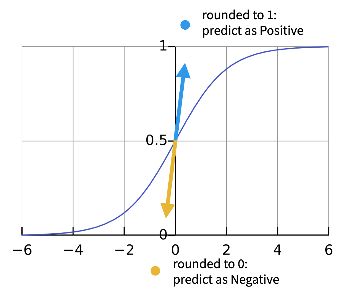
Another case could be Logistic regression, which various round can be reverse prediction.
Why is round different?
Let’s talk a little more about why this round is different.
Rounding as we usually perceive it means changing 0 ~ 4 to 0, and 5 ~ 9 to 10, as shown below image.
And in decimal units, is rounding to the nearest whole number by changing .0 ~ .4999.. to 0 and .5 ~ .9999.. to 1.
However, there are a number of mathematical interpretations of when exactly 0.5 , and when it is a negative number.

For example, round(-23.5) should produce -23 or -24?
Both are possible, depending on the mathematical interpretation and it’s called as rounding half up and rounding half down respectively. We can take this a step further and round both positive and negative numbers closer to zero, or vice versa.
This means that round(-23.5) will round to -23, and round(23.5) will round to 23, or round to -24 and 24, respectively. These are represented by the names Rounding half toward zero, Rounding half away from zero, respectively.
Finally, there are methods called Rounding half to even and Rounding half to odd, which mean that we want to consider the nearest integers to be even and odd, respectively.
In particular, the Rounding half to even method also goes by the names Convergent rounding, Statistician’s rounding, Dutch rounding, Gaussian rounding, and Bankers’ rounding, and is one of the official standard methods according to IEEE 754.
Bankers’ rounding
Bankers’s rounding, is default method in R , so Let’s breif a little bit more.
The image below shows the result of rounding from 0.0 to 2.0.

While this may seem like a good idea, there is actually a problem. Because .5 is unconditionally rounded to the next integer, there is an unconditional bias towards rounding to a “+ value”.
I don’t know the exact reason for this, but one theory is that the US IRS used to use this rounding to collect taxes and was sued for unfairly profiting by collecting more taxes from people who were .5 off, so they lost the case and changed to rounding to the nearest even (or odd) number to match the .5 rounding.
This means that by modifying the rounding as shown below, we can avoid the bias that was previously occurring.

The problem with different results
In recent years, industries in various domains, including pharmaceuticals and finance, have been trying to switch from “commercial” software such as SPSS, SAS and STATA to “open source” software such as Python, R and Julia .
And as rounding mentioned earlier, diffrent result issue by software has been also raised which can create problems in terms of reproducibility, uncertainty, accuracy, and traceability.
So if you’re utilizing multiple softwares, you should be aware of why they produce different results, and how you can use them to properly
CAMIS project

CAMIS stands for Comparing Analysis Method Implementations in Software.
This project compares the differences in softwares (or programming languages) and make standards to produce the same results.
The core area of the project is the “statistical computation” part, so most contributions come from the data science leaders who have strong understanding with it.
But CAMIS is also an open source project, that is not restricted and maintained with various people through regular discussions, collaboration, and sharing of project progress.
Below is one of the comparisons published on the CAMIS project’s webpage, which reviews how a one sample t-test is run with each software, what the results are, and how the results are compatible with each other.


The CAMIS project was started by members who interested in “SAS to R” in the medical and pharmaceutical industry. So it mainly focuses on R and SAS along major statistical data analysis, but recently it’s also working on how to use Python for data science in a broader domain of the industry.
Not only clasiccal methods such as Hypothesis tests, Regression analysis, but modern methods in data science such as Bayesian statistics, Causal inference and novel implementations of existing methods (e.g. MMRM) are topic of interest in project.
Sessions are increasingly appearing at multiple data science conferences, where many researchers and contributors are encouraged to promote, contribute and utilize it as a reference.
Finally, the CAMIS project is also collaborating with academia beyond the data science industry, as similar topics have been published in The American Statistician and Drug Information Association, among others.

The project is also currently working with students on a thesis entitled “A comparison of MMRM methodology in SAS and R software” and is open to collaborations and suggestions on other topics.
Summary
Various software used in data science. As the domain, the libraries or software used by an organization may be dependent on a particular language, which can sometimes be mixed with personal preferred methods. (in many cases, this doesn’t vary much at the level of the business)
However, if you’re not careful, the methods you use can lead to different results.
In this article, I’ve given you some examples of and reasons for differences in the methods used by different software for calculations, and introduced the CAMIS project, a research project that aims to minimize them to ensure consistency in data analysis.
If you use different software in your data analytics work, it’s a good idea to take a look at them to understand the differences and try to find the optimal method for your purposes,
And if you work in data science in the field, I highly recommend that you take an interstate in or contribute to the CAMIS project for a global collaborative experience.

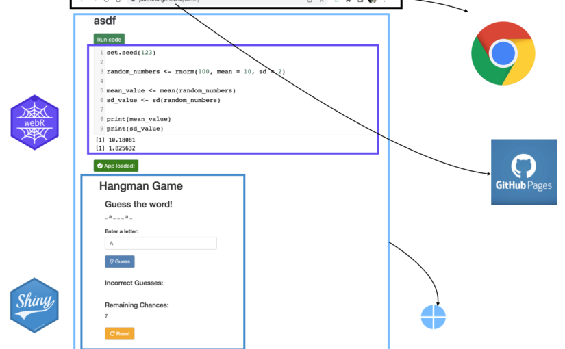
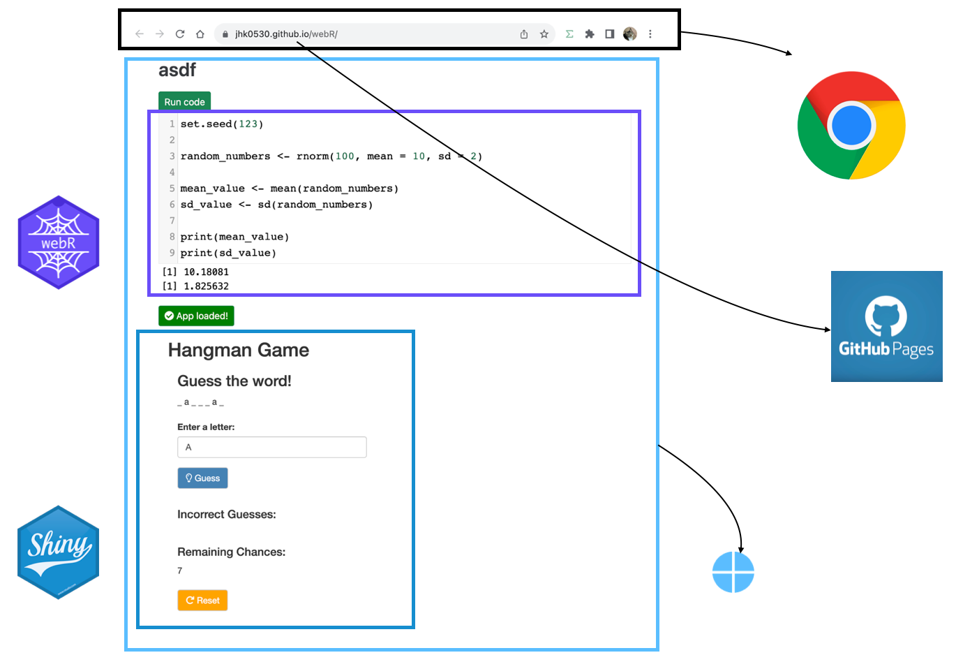
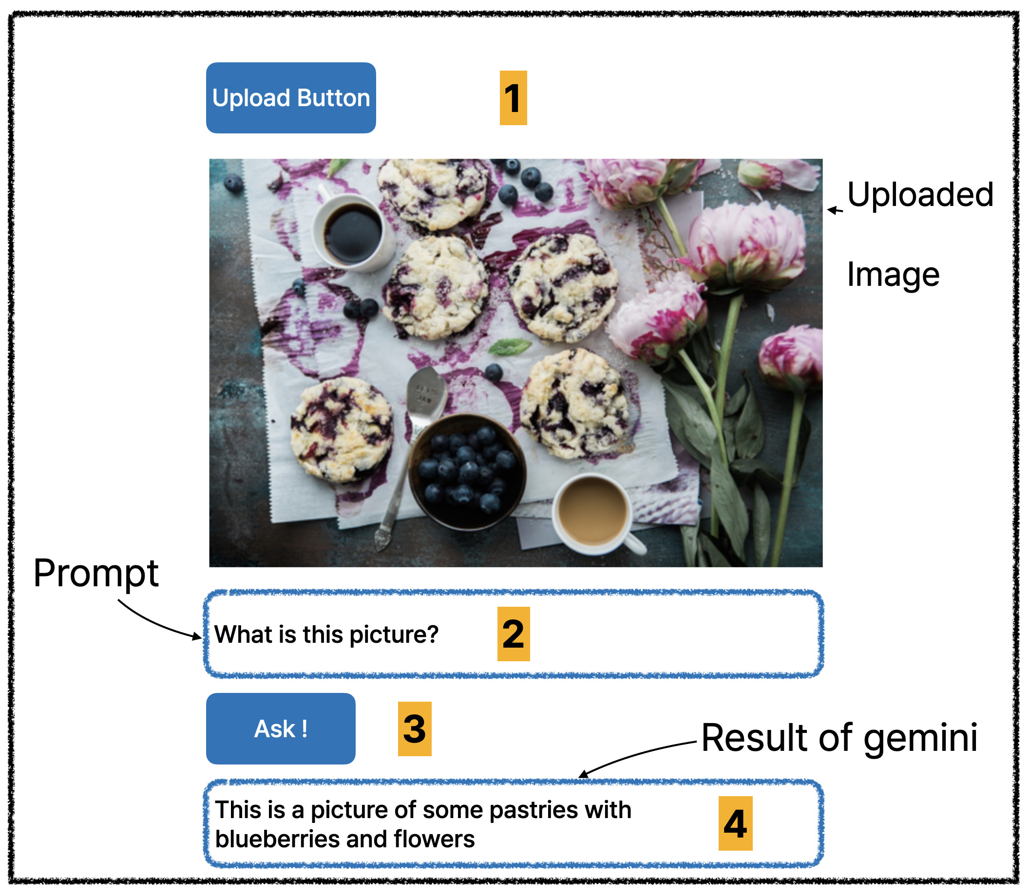 (Number is expected user flow)
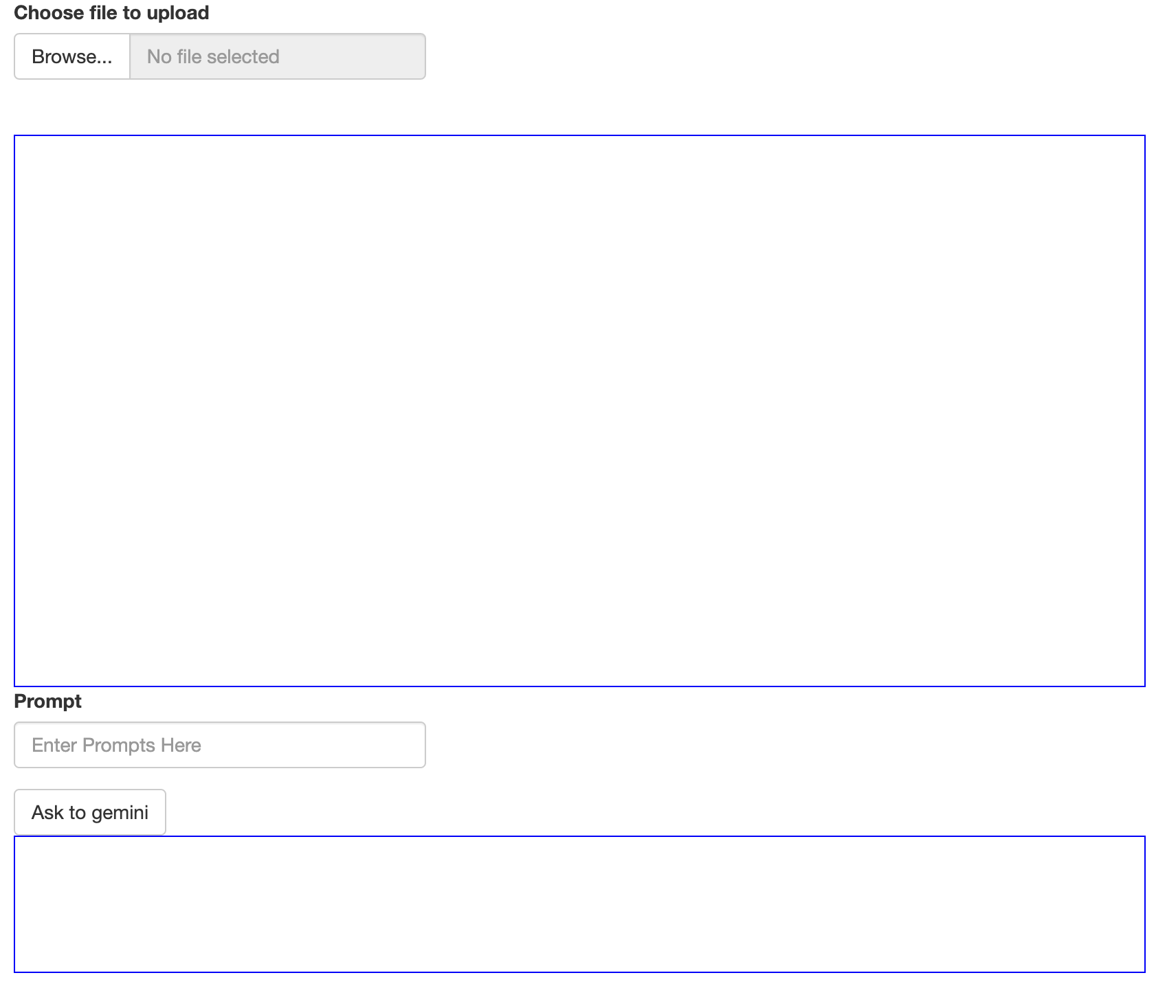
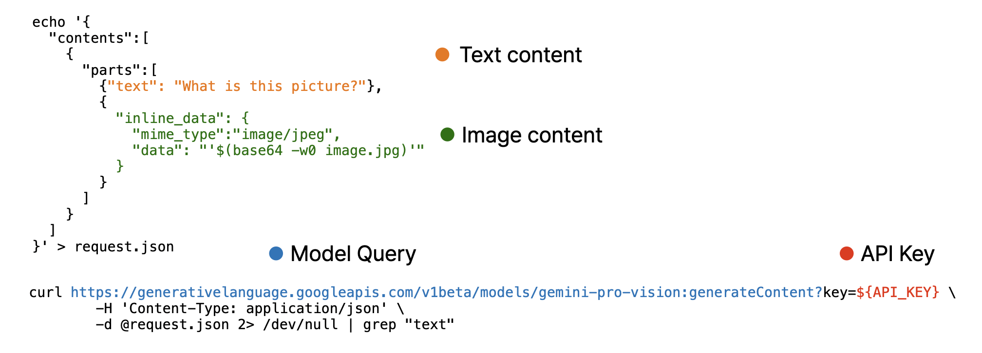
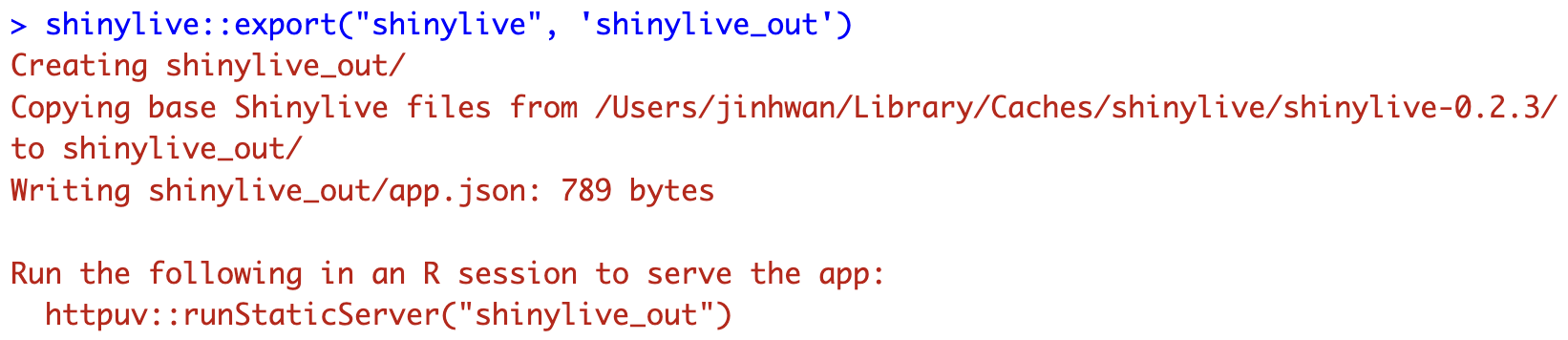
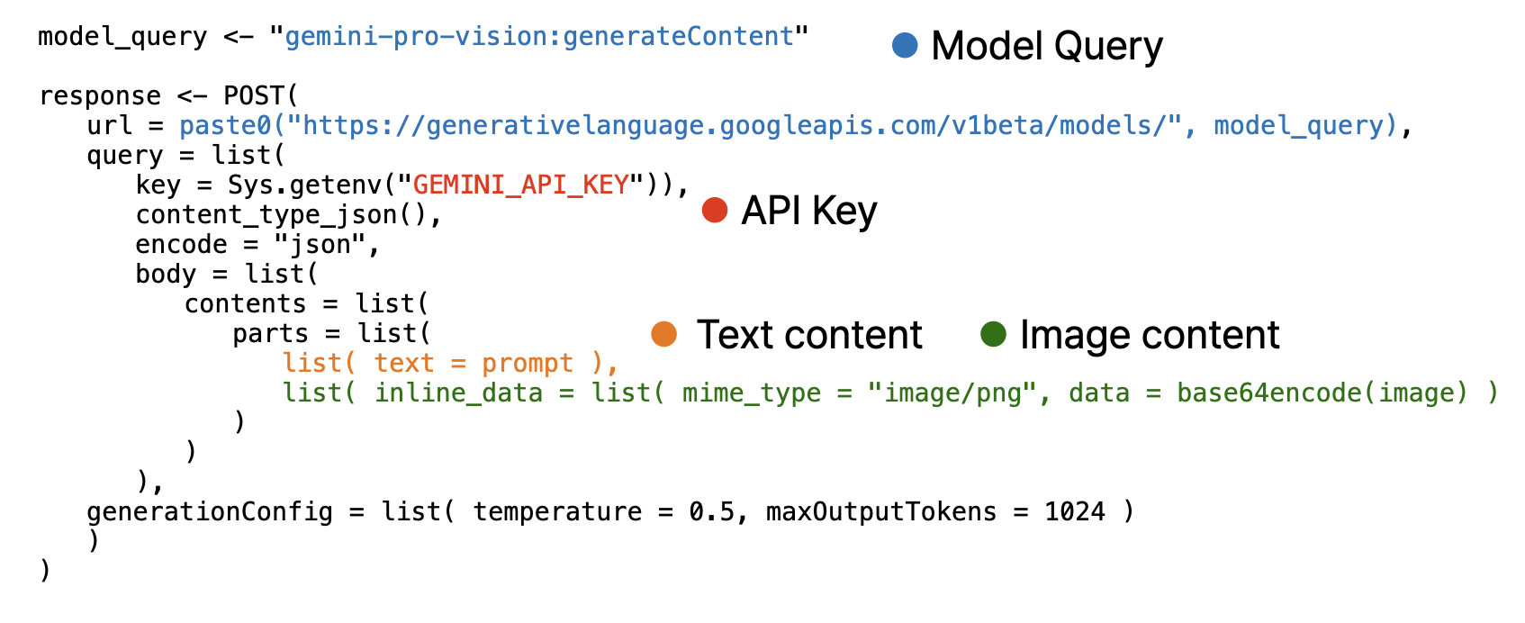 Note that, image must encoded as base64 using base64encode function and provided as separated list.


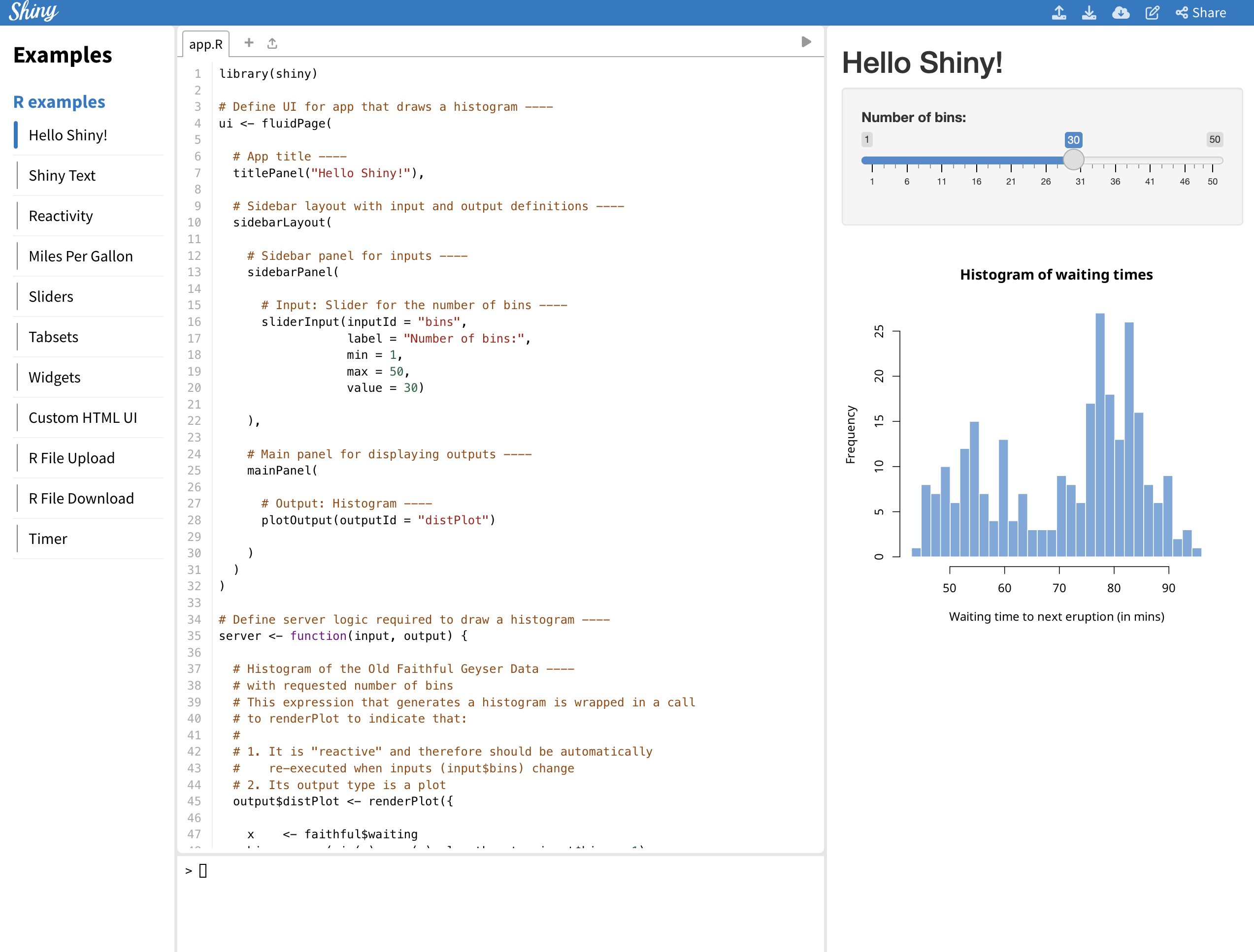
![Creating Standalone Apps from Shiny with Electron [2023, macOS M1]](https://r-posts.com/wp-content/uploads/2023/03/스크린샷-2023-03-14-오전-9.50.31-825x510.png)
 💡 I assume that…