shiny.webawesome brings Web Awesome to R Shiny through generated wrappers, reactive bindings, and a bundled runtime. It aims for complete component support while staying close enough to upstream that the Web Awesome docs and examples are directly useful in everyday package use.
CRAN | R-universe | Package website | Source repository
Background
shiny.webawesome started from a perceived gap: Shiny would benefit from a UI library that feels modern, visually polished, and broad enough to support a full app coherently. Web Awesome was a strong fit because it combines rich components, layout and styling utilities, and detailed upstream documentation with a standards-based web-components structure that is straightforward to track from R. That makes it easier for the package to stay close to upstream while still fitting naturally into Shiny.
The Whole Game
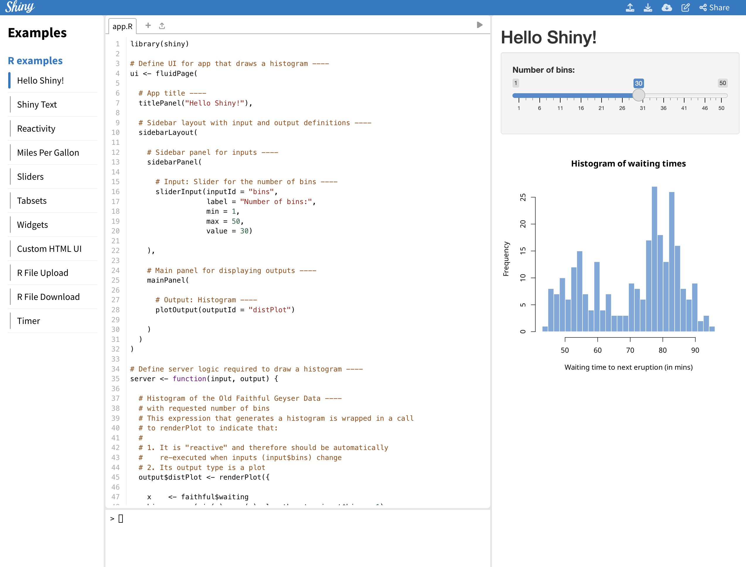
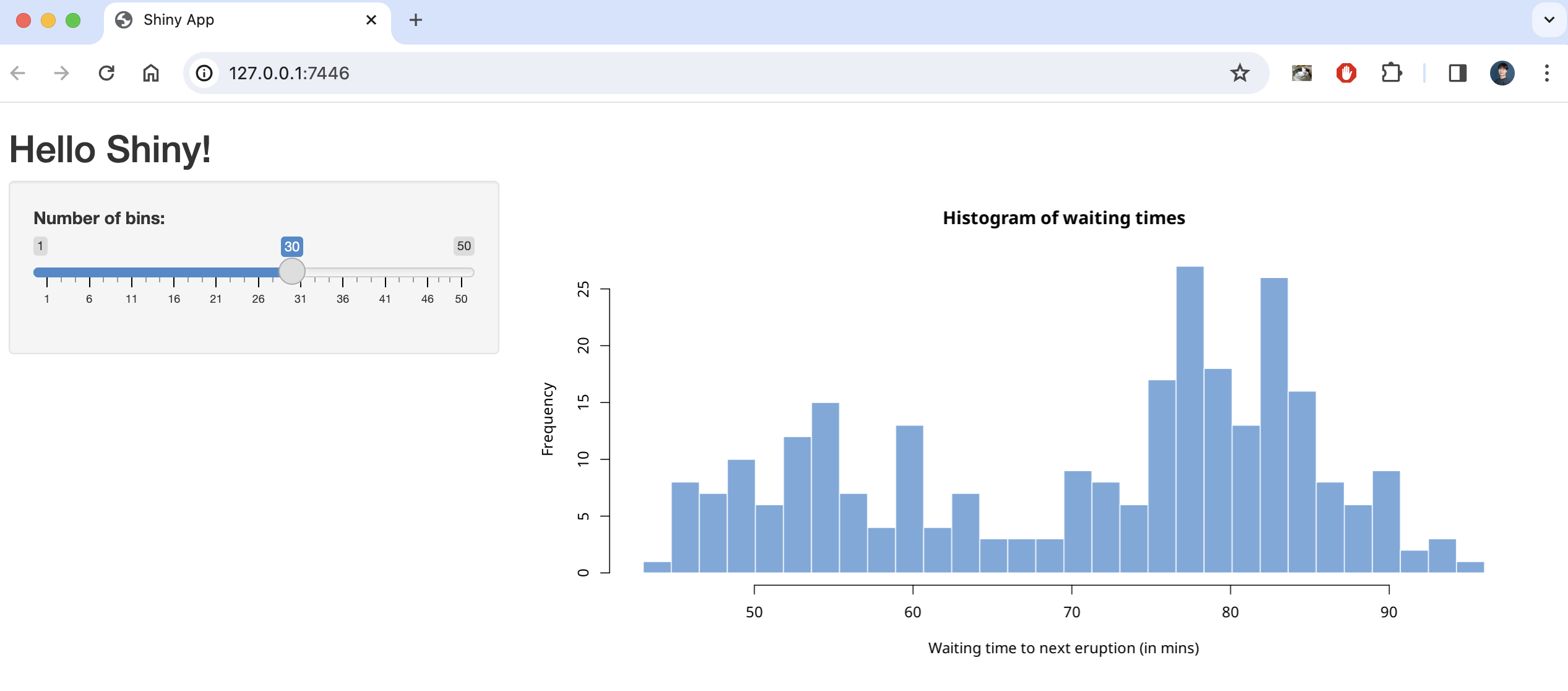
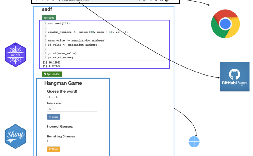
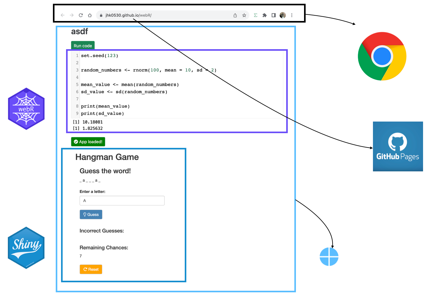
Here’s a screenshot of a simple, complete example app using shiny.webawesome. The full live app and code are available in an article at: https://mbanand.github.io/ghpages/announcement/..

This example showcases many of the facilities available in the package:
- a visually rich component library
- direct use of Web Awesome layout utilities such as
wa-stack,wa-cluster,wa-gap-*, andwa-align-*classes - styling through Web Awesome design tokens and classes such as
--wa-color-*,--wa-font-*, andwa-body-* - reactive Shiny input bindings
- helpers for calling methods on HTML elements, setting properties, and injecting simple JavaScript snippets
Design Philosophy
shiny.webawesome is designed to stay close to upstream Web Awesome. Most component wrappers are generated from Web Awesome metadata, which helps preserve upstream names, structure, and behavior while translating the interface into normal R conventions such as snake_case.
That close alignment has a practical benefit: when you want deeper details, examples, or component-specific guidance, you can usually go straight to the upstream Web Awesome documentation and apply what you find directly in shiny.webawesome. The package currently supports all Web Awesome components, so the upstream docs are a practical reference for day-to-day use.
To support the server-client model of Shiny, the package adds a small set of page and layout helpers, curated reactive bindings, and a narrow command layer for cases where browser-side interaction goes beyond the generated wrappers.
The result is a package with a clear default path. Use generated wrappers for ordinary UI, use bindings for meaningful reactive state, and reach for commands or small JavaScript glue when the app needs them.
Shiny Bindings
shiny.webawesome does not forward every browser event and every detail of component telemetry into Shiny. Much component state and interaction detail is better handled locally in the browser rather than turned into server messages. Consequently, the package exposes only a curated set of Shiny bindings that fit Shiny’s reactive model, with an emphasis on meaningful committed state rather than low-level browser event streams.
In the most common case, a binding publishes a durable semantic value. A select reports its current value, a dialog can report whether it is open, and a tree can report the currently selected item ids. The key idea is that Shiny receives the state the app actually cares about, not the raw event name that happened to produce it.
Some components are better treated as actions than values. A button is the clearest example: in Shiny, it behaves like a Shiny action input, with each click producing a new input event. A small number of components need both action semantics and a separate value. A dropdown, for example, may need to trigger reactivity on every choice, including repeated selections of the same item, while also exposing the latest selected value.
This design keeps reactive messaging to the server smaller, clearer, and easier to reason about. If an interaction belongs naturally in Shiny’s input model, shiny.webawesome will expose it as a binding. If it is more naturally a browser-side concern, it is usually a better fit for the command layer or a small amount of JavaScript glue.
For the full binding categories, semantics, and examples, see the package article: Shiny Bindings.
Command API
shiny.webawesome covers the most common interaction patterns through generated wrappers, Shiny bindings, and update helpers. But sometimes an app still needs to reach into a live browser element directly: set a property, call a method, or add a small browser-local JavaScript snippet.
For those cases, the package provides a narrow command API. The two main server-side helpers are wa_set_property() and wa_call_method(). They let Shiny code send one-way commands to a browser element identified by id, either by assigning a value to a live property or invoking a browser-side method.
If a component already has a binding or update helper, that should usually remain the first choice. The command layer is for the cases that fall just outside those built-in paths, where the simplest solution is still to tell the existing browser component to do one specific thing.
The package also includes wa_js() for a different kind of job: small, app-local JavaScript glue. That is useful when the missing piece is browser-side logic such as listening for an event, reading live component state, or publishing a derived value back to Shiny with Shiny.setInputValue().
For more detail and examples, see the package article: Command API.
Conclusion
shiny.webawesome brings a visually rich component library into Shiny while staying close to upstream Web Awesome. That combination gives polished components, useful layout and styling utilities, and a workflow where upstream documentation and examples remain directly relevant throughout app development.
For more examples, longer articles, and full reference material, see the package website: shiny-webawesome.org.


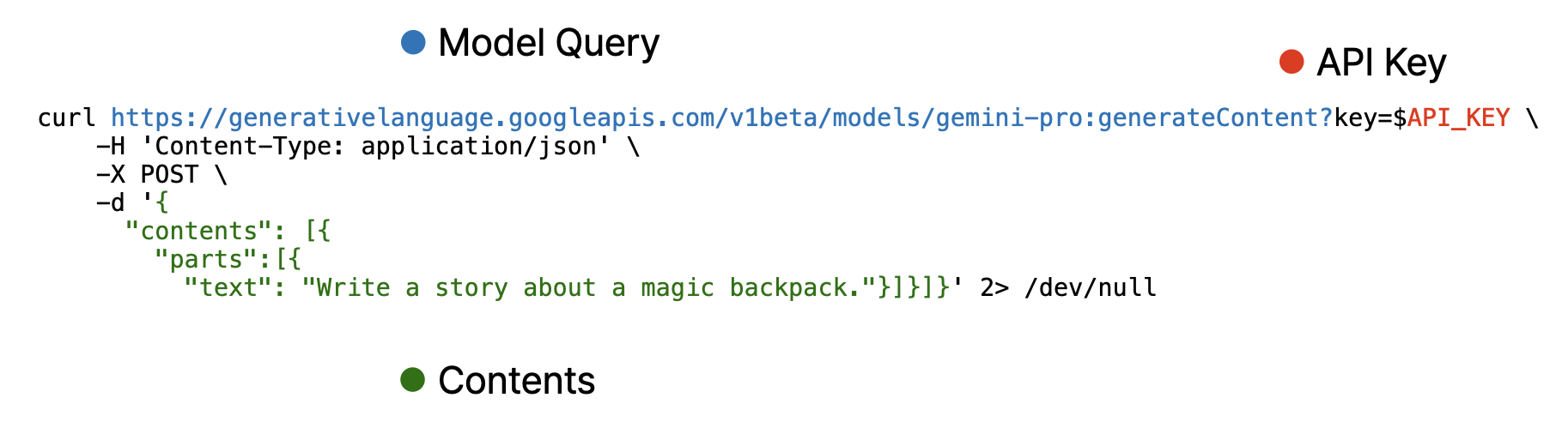
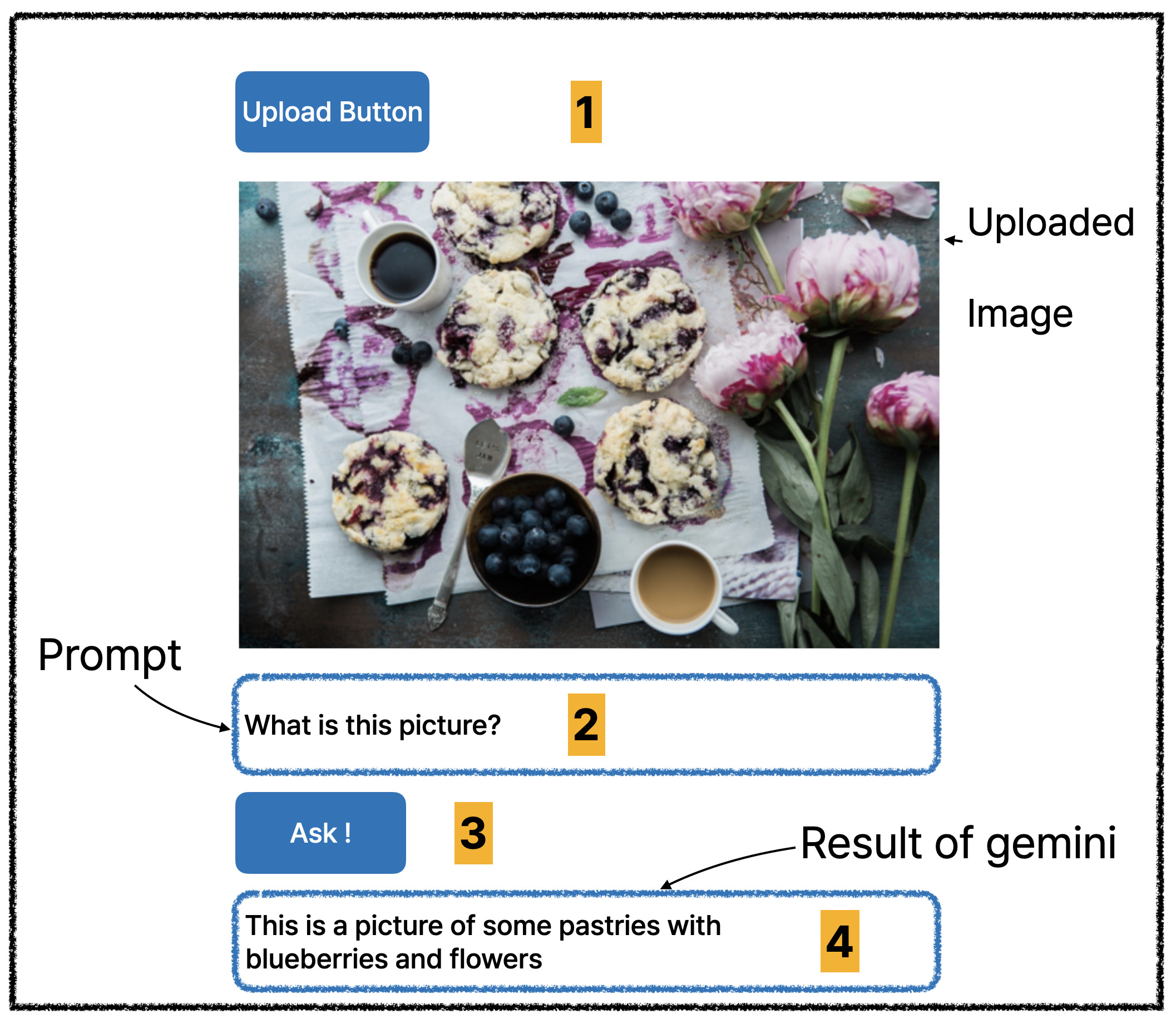 (Number is expected user flow)
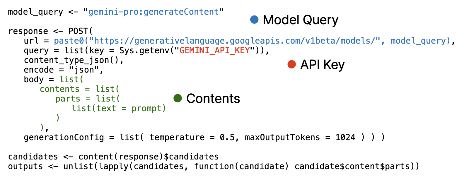
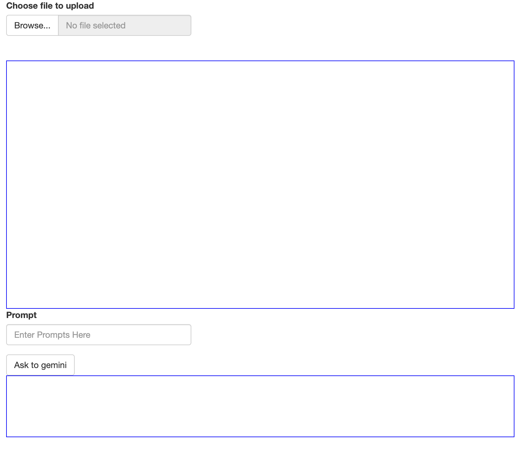
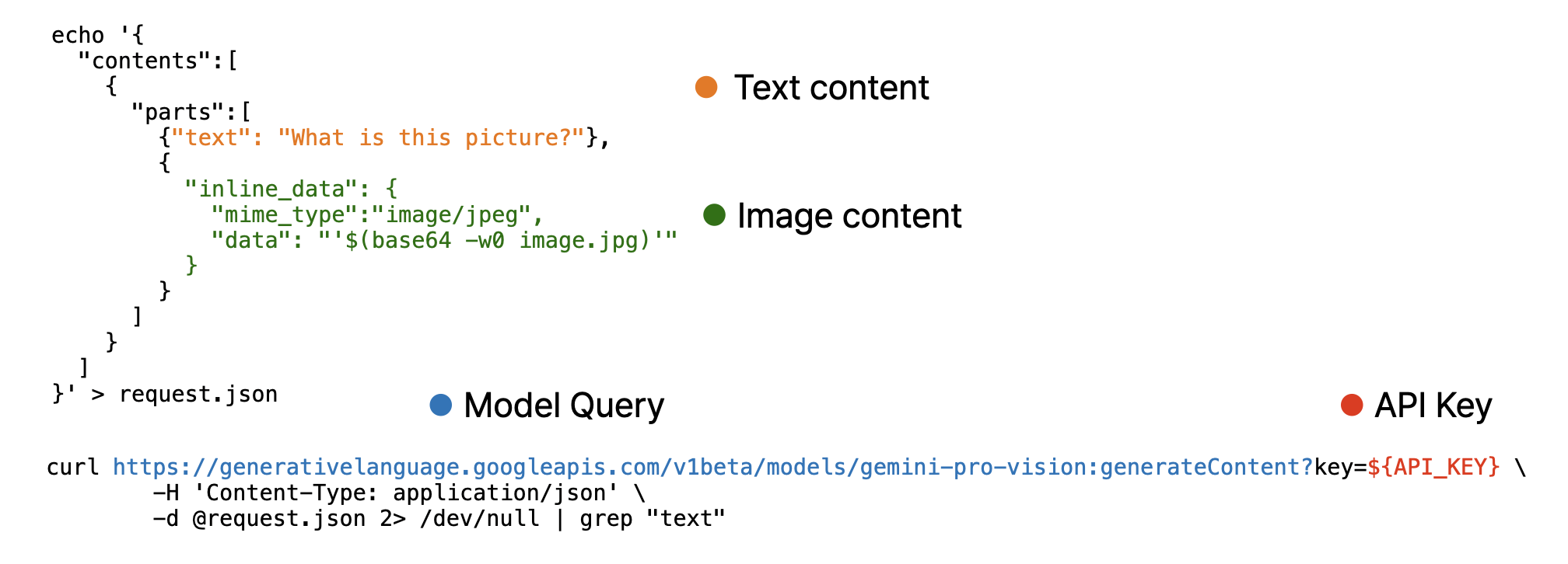
 Note that, image must encoded as base64 using base64encode function and provided as separated list.
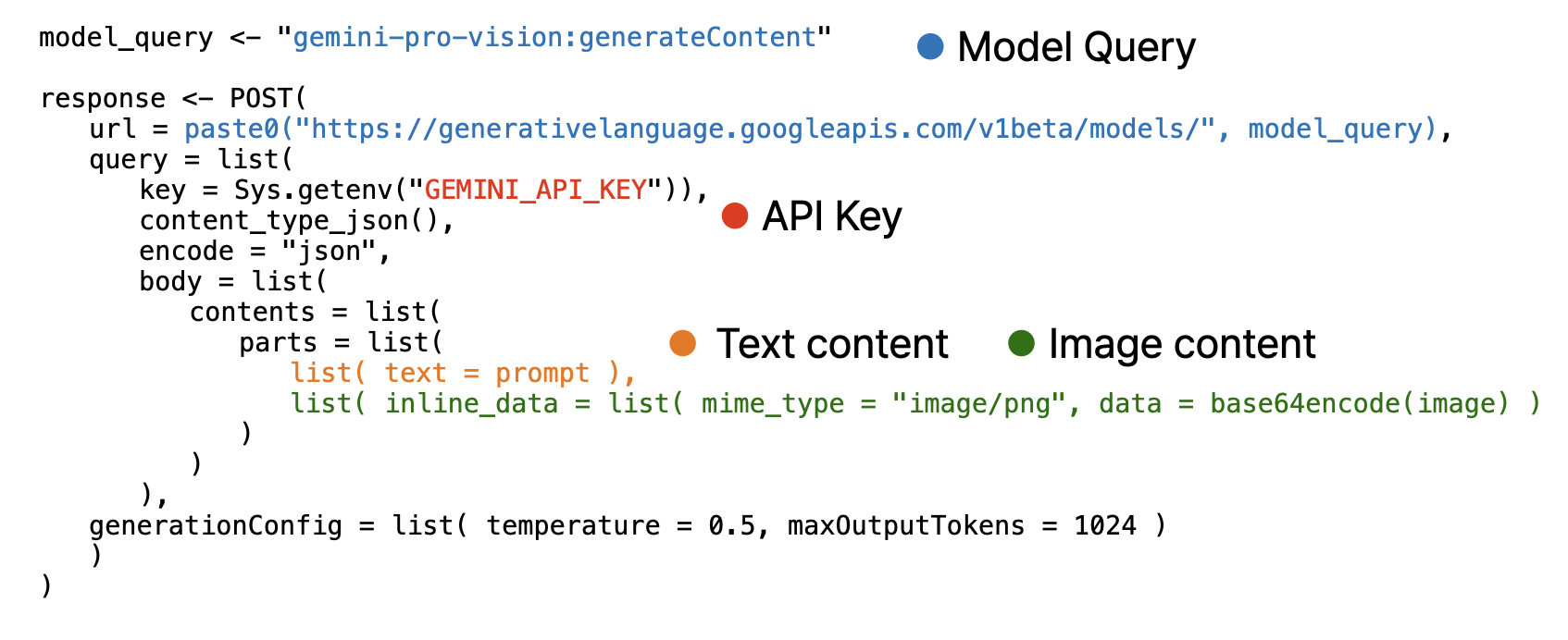


![Creating Standalone Apps from Shiny with Electron [2023, macOS M1]](http://r-posts.com/wp-content/uploads/2023/03/스크린샷-2023-03-14-오전-9.50.31-825x510.png)
 💡 I assume that…