This tutorial illustrates how to use the bwimge R package (Biagolini-Jr 2019) to describe patterns in images of natural structures. Digital images are basically two-dimensional objects composed by cells (pixels) that hold information of the intensity of three color channels (red, green and blue). For some file formats (such as png) another channel (the alpha channel) represents the degree of transparency (or opacity) of a pixel. If the alpha channel is equal to 0 the pixel will be fully transparent, if the alpha channel is equal to 1 the pixel will be fully opaque. Bwimage’s images analysis is based on transforming color intensity data to pure black-white data, and transporting the information to a matrix where it is possible to obtain a series of statistics data. Thus, the general routine of bwimage image analysis is initially to transform an image into a binary matrix, and secondly to apply a function to extract the desired information. Here, I provide examples and call attention to the following key aspects: i) transform an image to a binary matrix; ii) introduce distort images function; iii) demonstrate examples of bwimage application to estimate canopy openness; and iv) describe vertical vegetation complexity. The theoretical background of the available methods is presented in Biagolini & Macedo (2019) and in references cited along this tutorial. You can reproduce all examples of this tutorial by typing the given commands at the R prompt. All images used to illustrate the example presented here are in public domain. To download images, check out links in the Data availability section of this tutorial. Before starting this tutorial, make sure that you have installed and loaded bwimage, and all images are stored in your working directory.
install.packages("bwimage") # Download and install bwimage
library("bwimage") # Load bwimage package
setwd(choose.dir()) # Choose your directory. Remember to stores images to be analyzed in this folder.
Transform an image to a binary matrix
Transporting your image information to a matrix is the first step in any bwimage analysis. This step is critical for high quality analysis. The function threshold_color can be used to execute the thresholding process; with this function the averaged intensity of red, green and blue (or only just one channel if desired) is compared to a threshold (argument threshold_value). If the average intensity is less than the threshold (default is 50%) the pixel will be set as black, otherwise it will be white. In the output matrix, the value one represents black pixels, zero represents white pixels and NA represents transparent pixels. Figure 1 shows a comparison of threshold output when using all three channels in contrast to using just one channel (i.e. the effect of change argument channel).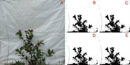
# RGB comparassion
imagename="VD01.JPG"
bush_rgb=threshold_color(imagename, channel = "rgb")
bush_r=threshold_color(imagename, channel = "r")
bush_g=threshold_color(imagename, channel = "g")
bush_b=threshold_color(imagename, channel = "b")

par(mfrow = c(2, 2), mar = c(0,0,0,0))
image(t(bush_rgb)[,nrow(bush_rgb):1], col = c("white","black"), xaxt = "n", yaxt = "n")
image(t(bush_r)[,nrow(bush_r):1], col = c("white","black"), xaxt = "n", yaxt = "n")
image(t(bush_g)[,nrow(bush_g):1], col = c("white","black"), xaxt = "n", yaxt = "n")
image(t(bush_b)[,nrow(bush_b):1], col = c("white","black"), xaxt = "n", yaxt = "n")
dev.off()
In this first example, the overall variations in thresholding are hard to detect with a simple visual inspection. This is because the way images were produced create a high contrast between the vegetation and the white background. Later in this tutorial, more information about this image will be presented. For a clear visual difference in the effect of change argument channel, let us repeat the thresholding process with two new images with more extreme color channel contrasts: sunflower (Figure 2), and Brazilian flag (Figure 3). 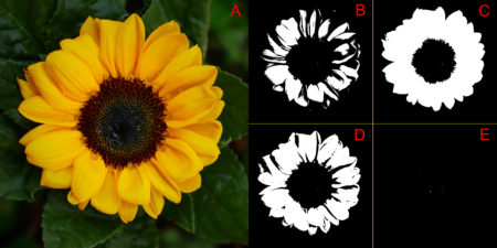
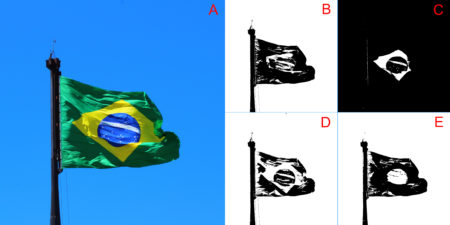
file_name="sunflower.JPG" # for figure 2
file_name="brazilian_flag.JPG" # for figure 03
Another important parameter that can affect output quality is the threshold value used to define if the pixel must be converted to black or white (i.e. the argument threshold_value in function threshold_color). Figure 4 compares the effect of using different threshold limits in the threshold output of the same bush image processed above.
# Threshold value comparassion
file_name="VD01.JPG"
bush_1=threshold_color(file_name, threshold_value = 0.1)
bush_2=threshold_color(file_name, threshold_value = 0.2)
bush_3=threshold_color(file_name, threshold_value = 0.3)
bush_4=threshold_color(file_name, threshold_value = 0.4)
bush_5=threshold_color(file_name, threshold_value = 0.5)
bush_6=threshold_color(file_name, threshold_value = 0.6)
bush_7=threshold_color(file_name, threshold_value = 0.7)
bush_8=threshold_color(file_name, threshold_value = 0.8)

par(mfrow = c(4, 2), mar = c(0,0,0,0))
image(t(bush_1)[,nrow(bush_1):1], col = c("white","black"), xaxt = "n", yaxt = "n")
image(t(bush_2)[,nrow(bush_2):1], col = c("white","black"), xaxt = "n", yaxt = "n")
image(t(bush_3)[,nrow(bush_3):1], col = c("white","black"), xaxt = "n", yaxt = "n")
image(t(bush_4)[,nrow(bush_4):1], col = c("white","black"), xaxt = "n", yaxt = "n")
image(t(bush_5)[,nrow(bush_5):1], col = c("white","black"), xaxt = "n", yaxt = "n")
image(t(bush_6)[,nrow(bush_6):1], col = c("white","black"), xaxt = "n", yaxt = "n")
image(t(bush_7)[,nrow(bush_7):1], col = c("white","black"), xaxt = "n", yaxt = "n")
image(t(bush_8)[,nrow(bush_8):1], col = c("white","black"), xaxt = "n", yaxt = "n")
dev.off()
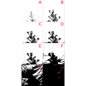
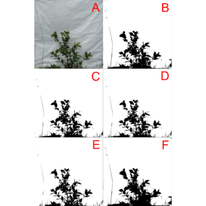
The bwimage package s threshold algorithm (described above) provides a simple, powerful and easy to understand process to convert colored images to a pure black and white scale. However, this algorithm was not designed to meet specific demands that may arise according to user applicability. Users interested in specific algorithms can use others R packages, such as auto_thresh_mask (Nolan 2019), to create a binary matrix to apply bwimage function. Below, we provide examples of how to apply four algorithms (IJDefault, Intermodes, Minimum, and RenyiEntropy) from the auto_thresh_mask function (auto_thresh_mask package – Nolan 2019), and use it to calculate vegetation density of the bush image (i.e. proportion of black pixels in relation to all pixels). I repeated the same analysis using bwimage algorithm to compare results. Figure 5 illustrates differences between image output from algorithms.# read tif image
img = ijtiff::read_tif("VD01.tif")
# IJDefault
IJDefault_mask= auto_thresh_mask(img, "IJDefault")
IJDefault_matrix = 1*!IJDefault_mask[,,1,1]
denseness_total(IJDefault_matrix)
# 0.1216476
# Intermodes
Intermodes_mask= auto_thresh_mask(img, "Intermodes")
Intermodes_matrix = 1*!Intermodes_mask[,,1,1]
denseness_total(Intermodes_matrix)
# 0.118868
# Minimum
Minimum_mask= auto_thresh_mask(img, "Minimum")
Minimum_matrix = 1*!Minimum_mask[,,1,1]
denseness_total(Minimum_matrix)
# 0.1133822
# RenyiEntropy
RenyiEntropy_mask= auto_thresh_mask(img, "RenyiEntropy")
RenyiEntropy_matrix = 1*!RenyiEntropy_mask[,,1,1]
denseness_total(RenyiEntropy_matrix)
# 0.1545827
# bWimage
bw_matrix=threshold_color("VD01.JPG")
denseness_total(bw_matrix)
# 0.1398836
The calculated vegetation density for each algorithm was:
| Algorithm | Vegetation density |
| IJDefault | 0.1334882 |
| Intermodes | 0.1199355 |
| Minimum | 0.1136603 |
| RenyiEntropy | 0.1599628 |
| Bwimage | 0.1397852 |
For a description of each algorithms, check out the documentation of function auto_thresh_mask and its references.
?auto_thresh_mask
par(mar = c(0,0,0,0)) ## Remove the plot margin
image(t(bw_matrix)[,nrow(bw_matrix):1], col = c("white","black"), xaxt = "n", yaxt = "n")
image(t(bw_matrix)[,nrow(bw_matrix):1], col = c("white","black"), xaxt = "n", yaxt = "n")
image(t(IJDefault_matrix)[,nrow(IJDefault_matrix):1], col = c("white","black"), xaxt = "n", yaxt = "n")
image(t(Intermodes_matrix)[,nrow(Intermodes_matrix):1], col = c("white","black"), xaxt = "n", yaxt = "n")
image(t(Minimum_matrix)[,nrow(Minimum_matrix):1], col = c("white","black"), xaxt = "n", yaxt = "n")
image(t(RenyiEntropy_matrix)[,nrow(RenyiEntropy_matrix):1], col = c("white","black"), xaxt = "n", yaxt = "n")
dev.off()
If you applied the above functions, you may have noticed that high resolution images imply in large R objects that can be computationally heavy (depending on your GPU setup). The argument compress_method from threshold_color and threshold_image_list functions can be used to reduce the output matrix. It reduces GPU usage and time necessary to run analyses. But it is necessary to keep in mind that by reducing resolution the accuracy of data description will be lowered. To compare different resamplings, from a figure of 2500×2500 pixels, check out figure 2 from Biagolini-Jr and Macedo (2019) . The available methods for image reduction are: i) frame_fixed, which resamples images to a desired target width and height; ii) proportional, which resamples the image by a given ratio provided in the argument “proportion”; iii) width_fixed, which resamples images to a target width, and also reduces the image height by the same factor. For instance, if the original file had 1000 pixels in width, and the new width_was set to 100, height will be reduced by a factor of 0.1 (100/1000); and iv) height_fixed, analogous to width_fixed, but assumes height as reference.
Distort images function
In many cases image distortion is intrinsic to image development, for instance global maps face a trade-off between distortion and the total amount of information that can be presented in the image. The bwimage package has two functions for distorting images (stretch and compress functions) which allow allow application of four different algorithms for mapping images, from circle to square and vice versa. Algorithms were adapted from Lambers (2016). Figure 6 compares image distortion of two images using stretch and compress functions, and all available algorithms.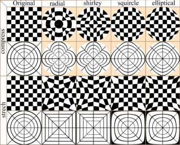
# Distortion images
chesstablet_matrix=threshold_color("chesstable.JPG")
target_matrix=threshold_color("target.JPG")

## Compress
# chesstablet_matrix
comp_cmr=compress(chesstablet_matrix,method="radial",background=0.5)
comp_cms=compress(chesstablet_matrix,method="shirley",background=0.5)
comp_cmq=compress(chesstablet_matrix,method="squircle",background=0.5)
comp_cme=compress(chesstablet_matrix,method="elliptical",background=0.5)

# target_matrix
comp_tmr=compress(target_matrix,method="radial",background=0.5)
comp_tms=compress(target_matrix,method="shirley",background=0.5)
comp_tmq=compress(target_matrix,method="squircle",background=0.5)
comp_tme=compress(target_matrix,method="elliptical",background=0.5)


## stretch
# chesstablet_matrix
stre_cmr=stretch(chesstablet_matrix,method="radial")
stre_cms=stretch(chesstablet_matrix,method="shirley")
stre_cmq=stretch(chesstablet_matrix,method="squircle")
stre_cme=stretch(chesstablet_matrix,method="elliptical")

# target_matrix
stre_tmr=stretch(target_matrix,method="radial")
stre_tms=stretch(target_matrix,method="shirley")
stre_tmq=stretch(target_matrix,method="squircle")
stre_tme=stretch(target_matrix,method="elliptical")

# Plot
par(mfrow = c(4,5), mar = c(0,0,0,0))
image(t(chesstablet_matrix)[,nrow(chesstablet_matrix):1], col = c("white","bisque","black"), xaxt = "n", yaxt = "n")
image(t(comp_cmr)[,nrow(comp_cmr):1], col = c("white","bisque","black"), xaxt = "n", yaxt = "n")
image(t(comp_cms)[,nrow(comp_cms):1], col = c("white","bisque","black"), xaxt = "n", yaxt = "n")
image(t(comp_cmq)[,nrow(comp_cmq):1], col = c("white","bisque","black"), xaxt = "n", yaxt = "n")
image(t(comp_cme)[,nrow(comp_cme):1], col = c("white","bisque","black"), xaxt = "n", yaxt = "n")
image(t(target_matrix)[,nrow(target_matrix):1], col = c("white","bisque","black"), xaxt = "n", yaxt = "n")
image(t(comp_tmr)[,nrow(comp_tmr):1], col = c("white","bisque","black"), xaxt = "n", yaxt = "n")
image(t(comp_tms)[,nrow(comp_tms):1], col = c("white","bisque","black"), xaxt = "n", yaxt = "n")
image(t(comp_tmq)[,nrow(comp_tmq):1], col = c("white","bisque","black"), xaxt = "n", yaxt = "n")
image(t(comp_tme)[,nrow(comp_tme):1], col = c("white","bisque","black"), xaxt = "n", yaxt = "n")
image(t(chesstablet_matrix)[,nrow(chesstablet_matrix):1], col = c("white","bisque","black"), xaxt = "n", yaxt = "n")
image(t(stre_cmr)[,nrow(stre_cmr):1], col = c("white","black"), xaxt = "n", yaxt = "n")
image(t(stre_cms)[,nrow(stre_cms):1], col = c("white","black"), xaxt = "n", yaxt = "n")
image(t(stre_cmq)[,nrow(stre_cmq):1], col = c("white","black"), xaxt = "n", yaxt = "n")
image(t(stre_cme)[,nrow(stre_cme):1], col = c("white","black"), xaxt = "n", yaxt = "n")
image(t(target_matrix)[,nrow(target_matrix):1], col = c("white","black"), xaxt = "n", yaxt = "n")
image(t(stre_tmr)[,nrow(stre_tmr):1], col = c("white","black"), xaxt = "n", yaxt = "n")
image(t(stre_tms)[,nrow(stre_tms):1], col = c("white","black"), xaxt = "n", yaxt = "n")
image(t(stre_tmq)[,nrow(stre_tmq):1], col = c("white","black"), xaxt = "n", yaxt = "n")
image(t(stre_tme)[,nrow(stre_tme):1], col = c("white","black"), xaxt = "n", yaxt = "n")
dev.off()
Application examples
Estimate canopy openness
Canopy openness is one of the most common vegetation parameters of interest in field ecology surveys. Canopy openness can be calculated based on pictures on the ground or by an aerial system e.g. (Díaz and Lencinas 2018). Next, we demonstrate how to estimate canopy openness, using a picture taken on the ground. The photo setup is described in Biagolini-Jr and Macedo (2019). Canopy closure can be calculated by estimating the total amount of vegetation in the canopy. Canopy openness is equal to one minus the canopy closure. You can calculate canopy openness for the canopy image example (provide by bwimage package) using the following code:canopy=system.file("extdata/canopy.JPG",package ="bwimage")
canopy_matrix=threshold_color(canopy,"jpeg", compress_method="proportional",compress_rate=0.1)
1-denseness_total(canopy_matrix) # canopy openness
For users interested in deeper analyses of canopy images, I also recommend the caiman package.Describe vertical vegetation complexity
There are several metrics to describe vertical vegetation complexity that can be performed using a picture of a vegetation section against a white background, as described by Zehm et al. (2003). Part of the metrics presented by these authors were implemented in bwimage, and the following code shows how to systematically extract information for a set of 12 vegetation pictures. A description of how to obtain a digital image for the following methods is presented in Figure 7.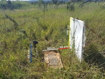
files_names= c("VD01.JPG", "VD02.JPG", "VD03.JPG", "VD04.JPG", "VD05.JPG", "VD06.JPG", "VD07.JPG", "VD08.JPG", "VD09.JPG", "VD10.JPG", "VD11.JPG", "VD12.JPG")

image_matrix_list=threshold_image_list(files_names, filetype = "jpeg",compress_method = "frame_fixed",target_width = 500,target_height=500)
Once you obtain the list of matrices, you can use a loop or apply family functions to extract information from all images and save them into objects or a matrix. I recommend storing all image information in a matrix, and exporting this matrix as a csv file. It is easier to transfer information to another database software, such as an excel sheet. Below, I illustrate how to apply functions denseness_total, heigh_propotion_test, and altitudinal_profile, to obtain information on vegetation density, a logical test to calculate the height below which 75% of vegetation denseness occurs, and the average height of 10 vertical image sections and its SD (note: sizes expressed in cm).
answer_matrix=matrix(NA,ncol=4,nrow=length(image_matrix_list))
row.names(answer_matrix)=files_names
colnames(answer_matrix)=c("denseness", "heigh 0.75", "altitudinal mean", "altitudinal SD")
# Loop to analyze all images and store values in the matrix
for(i in 1:length(image_matrix_list)){
  answer_matrix[i,1]=denseness_total(image_matrix_list[[i]])
  answer_matrix[i,2]=heigh_propotion_test(image_matrix_list[[i]],proportion=0.75, height_size= 100)
  answer_matrix[i,3]=altitudinal_profile(image_matrix_list[[i]],n_sections=10, height_size= 100)[[1]]
  answer_matrix[i,4]=altitudinal_profile(image_matrix_list[[i]],n_sections=10, height_size= 100)[[2]]
}
Finally, we analyze information of holes data (i.e. vegetation gaps), in 10 image lines equally distributed among image (Zehm et al. 2003). For this purpose, we use function altitudinal_profile. Sizes are expressed in number of pixels.# set a number of samples
nsamples=10
# create a matrix to receive calculated values
answer_matrix2=matrix(NA,ncol=7,nrow=length(image_matrix_list)*nsamples)
colnames(answer_matrix2)=c("Image name", "heigh", "N of holes", "Mean size", "SD","Min","Max")
# Loop to analyze all images and store values in the matrix
for(i in 1:length(image_matrix_list)){
for(k in 1:nsamples){
line_heigh= k* length(image_matrix_list[[i]][,1])/nsamples
aux=hole_section_data(image_matrix_list[[i]][line_heigh,] )
answer_matrix2[((i-1)*nsamples)+k ,1]=files_names[i]
answer_matrix2[((i-1)*nsamples)+k ,2]=line_heigh
answer_matrix2[((i-1)*nsamples)+k ,3:7]=aux
}}
write.table(answer_matrix2, file = "Image_data2.csv", sep = ",", col.names = NA, qmethod = "double")
Data availability
To download images access: https://figshare.com/articles/image_examples_for_bwimage_tutorial/9975656References
Biagolini-Jr C (2019) bwimage: Describe Image Patterns in Natural Structures. https://cran.r-project.org/web/packages/bwimage/index.htmlBiagolini-Jr C, Macedo RH (2019) bwimage: A package to describe image patterns in natural structures. F1000Research 8 https://f1000research.com/articles/8-1168
Díaz GM, Lencinas JD (2018) Model-based local thresholding for canopy hemispherical photography. Canadian Journal of Forest Research 48:1204-1216 https://www.nrcresearchpress.com/doi/abs/10.1139/cjfr-2018-0006
Lambers M (2016) Mappings between sphere, disc, and square. Journal of Computer Graphics Techniques Vol 5:1-21 http://jcgt.org/published/0005/02/01/paper-lowres.pdf
Nolan R (2019) autothresholdr: An R Port of the ‘ImageJ’ Plugin ‘Auto Threshold. https://cran.r-project.org/web/packages/autothresholdr/
Zehm A, Nobis M, Schwabe A (2003) Multiparameter analysis of vertical vegetation structure based on digital image processing. Flora-Morphology, Distribution, Functional Ecology of Plants 198:142-160 https://doi.org/10.1078/0367-2530-00086