Everyday, around 9 pm, I get fresh portion of the Netflix Top movies / TV shows. I’ve been doing this for more than two months and decided to show the first results answering following questions:
How many movies / TV shows make the Top?
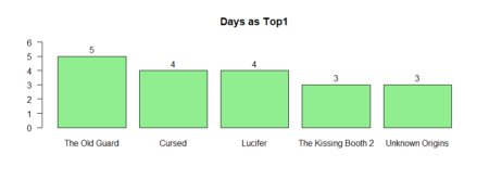
What movie was the longest #1 on Netflix?
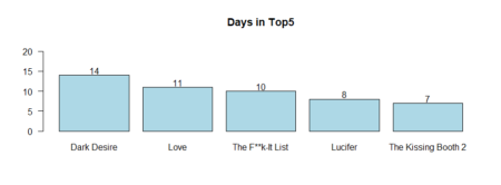
What movie was the longest in Tops?
For how many days movies / TV shows stay in Tops and as #1?
To have a try to plot all this up and down zigzags…
I took 60 days span (almost all harvest so far) and Top5 overall, not Top10, in each category to talk about really the most popular and trendy.
So, let`s count how many movies made the Top5, I mean it is definitely less than 5 *60…
library(tidyverse)
library (stats)
library (gt)
fjune <- read_csv("R/movies/fjune.csv")
#wrangle raw data - reverse (fresh date first), take top 5, take last 60 days
fjune_dt %>% rev () %>% slice (1:5) %>% select (1:60)

#gather it together and count the number of unique titles
fjune_dt_gathered <- gather (fjune_dt)
colnames (fjune_dt_gathered) <- c("date", "title")
unique_fjune_gathered <- unique (fjune_dt_gathered$title)

str (unique_fjune_gathered)
#chr [1:123] "Unknown Origins" "The Debt Collector 2" "Lucifer" "Casino Royale"
OK, it is 123 out of 300. Now, it is good to have distribution in each #1 #2 #3 etc.
t_fjune_dt <- as.data.frame (t(fjune_dt),stringsAsFactors = FALSE)
# list of unique titles in each #1 #2 #3etc. for each day
unique_fjune <- sapply (t_fjune_dt, unique)

# number of unique titles in each #1 #2 #3 etc.
n_unique_fjune <- sapply (unique_fjune, length)
n_unique_fjune <- setNames (n_unique_fjune, c("Top1", "Top2", "Top3", "Top4", "Top5"))

n_unique_fjune
Top1 Top2 Top3 Top4 Top5
32   45   45   52   49
What movie was the longest in Tops / #1?# Top5 table_fjune_dt5 <- sort (table (fjune_dt_gathered$title), decreasing = T) # Top1 table_fjune_dt1 <- sort (table (t_fjune_dt$V1), decreasing = T) # plotting the results bb5 <- barplot (table_fjune_dt5 [1:5], ylim=c(0,22), main = "Days in Top5", las = 1, col = 'light blue') text(bb5,table_fjune_dt5 [1:5] +1.2,labels=as.character(table_fjune_dt5 [1:5])) bb1 <- barplot (table_fjune_dt1 [1:5], main = "Days as Top1", las = 1, ylim=c(0,6), col = 'light green') text(bb1,table_fjune_dt1 [1:5] +0.5, labels=as.character(table_fjune_dt1 [1:5]))
Let`s weight and rank (1st = 5, 2nd = 4, 3rd = 3 etc.) Top 5 movies / TV shows during last 60 days.
i<- (5:1)
fjune_dt_gathered5 <- cbind (fjune_dt_gathered, i)
fjune_dt_weighted % group_by(title) %>% summarise(sum = sum (i)) %>% arrange (desc(sum))
top_n (fjune_dt_weighted, 10) %>% gt ()
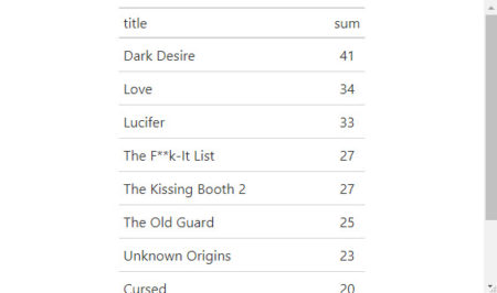
As we see the longer movies stays in Top the better rank they have with simple weighting meaning “lonely stars”, which got the most #1, draw less top attention through the time span.
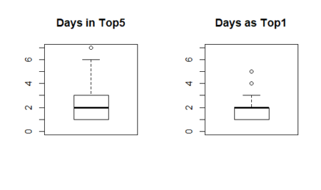
Average days in top
av_fjune_dt5 <- round (nrow (fjune_dt_gathered) / length (unique_fjune_gathered),1) # in Top5
av_fjune_dt1 <- round (nrow (t_fjune_dt) / length (unique_fjune$V1),1) #as Top1

cat("Average days in top5: ", av_fjune_dt5, "\n")
cat("Average days as top1: ", av_fjune_dt1)
#Average days in top5: 2.4
#Average days as top1: 1.9
Average days in top distributionas5 <- as.data.frame (table_fjune_dt5, stringsAsFActrors=FALSE) as1 <- as.data.frame (table_fjune_dt1, stringsAsFActrors=FALSE) par (mfcol = c(1,2)) boxplot (as5$Freq, ylim=c(0,7), main = "Days in Top5") boxplot (as1$Freq, ylim=c(0,7), main = "Days as Top1")
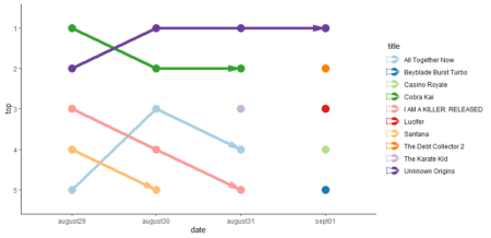
And now, let`s try to plot Top5 movies / TV shows daily changes.
I played with different number of days and picked 4 – with longer span I had less readable plots since every new day brings new comers into the Top with its own line, position in the legend, and, ideally its own color.
fjune_dt_gathered55 <- fjune_dt_gathered5 %>% slice (1:20) %>% rev ()
ggplot(fjune_dt_gathered55)+ aes (x=date, y=i, group = title) + geom_line (aes (color = title), size = 2) +
geom_point (aes (color = title), size = 5)+ theme_classic()+
theme(legend.position="right")+ylab("top")+ ylim ("5", "4", "3", "2", "1")+
geom_line(aes(colour = title), arrow = arrow(angle = 15, ends = "last", type = "closed"))+scale_color_brewer(palette="Paired")
where can I get the dataset of every month like this, please?
if you want to follow my steps – create it
Hi Andrew,
Where did you get the dataset that you used in this post?
Hi there,
I created the dataset. As I said: Everyday, around 9 pm…Basic rvest commands
Where does the data come from?
Hi, [email protected]! Where did you come from?)