By Huey Fern Tay with Greg Page
When are two variables too related to one another to be used together in a linear regression model? Should the maximum acceptable correlation be 0.7? Or should the rule of thumb be 0.8? There is actually no single, ‘one-size-fits-all’ answer to this question.
As an alternative to using pairwise correlations, an analyst can examine the variance inflation factor, or VIF, associated with each of the numeric input variables. Sometimes, however, pairwise correlations, and even VIF scores, do not tell the entire picture.
Consider this correlation matrix created from a Los Angeles Airbnb dataset.
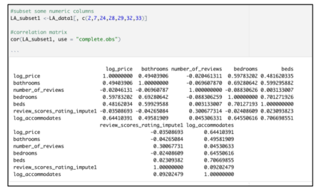
Two item pairs identified in the correlation matrix above have a strong correlation value:
· Beds + log_accommodates (r= 0.701)
· Beds + bedrooms (r= 0.706)
Based on one school of thought, these correlation values are cause for concern; meanwhile, other sources suggest that such values are nothing to be worried about.
The variance inflation factor, which is used to detect the severity of multicollinearity, does not suggest anything unusual either.
library(car)
vif(model_test)
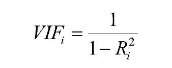
The VIF for each potential input variable is found by making a separate linear regression model, in which the variable being scored serves as the outcome, and the other numeric variables are the predictors. The VIF score for each variable is found by applying this formula:
When the other numeric inputs explain a large percentage of the variability in some other variable, then that variable will have a high VIF. Some sources will tell you that any VIF above 5 means that a variable should not be used in a model, whereas other sources will say that VIF values below 10 are acceptable. None of the vif() results here appear to be problematic, based on standard cutoff thresholds.
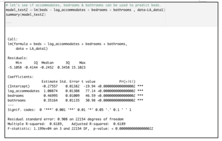
Based on the vif() results shown above, plus some algebraic manipulation of the VIF formula, we can know that a model that predicts beds as the outcome variable, using log_accommodates, bedrooms, and bathrooms as the inputs, has an r-squared of just a little higher than 0.61. That is verified with the model shown below:
But look at what happens when we build a multi-linear regression model predicting the price of an Airbnb property listing.
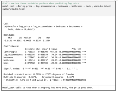
The model summary hints at a problem because the coefficient for beds is negative. The proper interpretation for each coefficient in this linear model is the way that log_price will be impacted by a one-unit increase in that input, with all other inputs held constant.
Literally, then, this output indicates that having more beds within a house or apartment will make its rental value go down, when all else is held constant. That not only defies our common sense, but it also contradicts something that we already know to be the case — that bed number and log_price are positively associated. Indeed, the correlation matrix shown above indicates a moderately-strong linear relationship between these values, of 0.4816.
After dropping ‘beds’ from the original model, the adjusted R-squared declines only marginally, from 0.4878 to 0.4782.
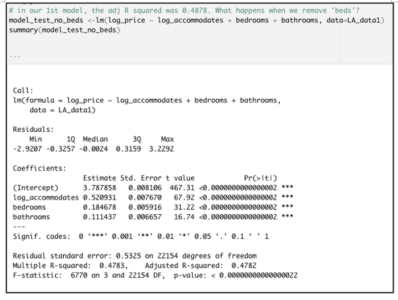
This tiny decline in adjusted r-squared is not worrisome at all. The very low p-value associated with this model’s F-statistic indicates a highly significant overall model. Moreover, the signs of the coefficients for each of these inputs are consistent with the directionality that we see in the original correlation matrix.
Moreover, we still need to include other important variables that determine real estate pricing e.g. location and property type. After factoring in these categories along with other considerations such as pool availability, cleaning fee, and pet-friendly options, the model’s adjusted R-squared value is pushed to 0.6694. In addition, the residual standard error declines from 0.5276 in the original model to 0.4239.
Long story short: we cannot be completely reliant on rules of thumb, or even cutoff thresholds from textbooks, when evaluating the multicollinearity risk associated with specific numeric inputs. We must also examine model coefficients’ signs. When a coefficient’s sign “flips” from the direction that we should expect, based on that variable’s correlation with the response variable, that can also indicate that our model coefficients are impacted by multicollinearity.
Data source: Inside Airbnb
One thought on “Detecting multicollinearity — it’s not that easy sometimes”