Factor Analysis in R workshop

Join our workshop on Factor Analysis in R, which is a part of our workshops for Ukraine series! 

Here’s some more info: 

Title: Factor Analysis in R

Date: Thursday, February 1st, 18:00 – 20:00 CET (Rome, Berlin, Paris timezone)

Speaker: Gagan Atreya is a quantitative social scientist and data science consultant based in Los Angeles, California. He has graduate degrees in Experimental Psychology and Quantitative Political Science from The College of William & Mary in Virginia and The University of Minnesota respectively. He has multiple years of experience in data analysis and visualization in the social sciences – both as a researcher and a consultant with faculty and researchers around the world. You can find him in Bluesky at @gaganatreya.bsky.social.

Description: This workshop will go through the basics of Exploratory and Confirmatory Factor Analysis in the R programming language. Factor Analysis is a valuable statistical technique widely used in Psychology, Economics, Political Science, and related disciplines that allows us to uncover the underlying structure of our data by reducing it to coherent factors. The workshop will heavily (but not exclusively) utilize the “psych” and “lavaan” packages in R. Although open to everyone, a beginner level familiarity with R and some background/interest in survey data analysis will be ideal to make the most out of this workshop.

Minimal registration fee: 20 euro (or 20 USD or 800 UAH)


How can I register?


  • Save your donation receipt (after the donation is processed, there is an option to enter your email address on the website to which the donation receipt is sent)

  • Fill in the registration form, attaching a screenshot of a donation receipt (please attach the screenshot of the donation receipt that was emailed to you rather than the page you see after donation).

If you are not personally interested in attending, you can also contribute by sponsoring a participation of a student, who will then be able to participate for free. If you choose to sponsor a student, all proceeds will also go directly to organisations working in Ukraine. You can either sponsor a particular student or you can leave it up to us so that we can allocate the sponsored place to students who have signed up for the waiting list.


How can I sponsor a student?


  • Save your donation receipt (after the donation is processed, there is an option to enter your email address on the website to which the donation receipt is sent)

  • Fill in the sponsorship form, attaching the screenshot of the donation receipt (please attach the screenshot of the donation receipt that was emailed to you rather than the page you see after the donation). You can indicate whether you want to sponsor a particular student or we can allocate this spot ourselves to the students from the waiting list. You can also indicate whether you prefer us to prioritize students from developing countries when assigning place(s) that you sponsored.


If you are a university student and cannot afford the registration fee, you can also sign up for the waiting list here. (Note that you are not guaranteed to participate by signing up for the waiting list).


You can also find more information about this workshop series,  a schedule of our future workshops as well as a list of our past workshops which you can get the recordings & materials here.


Looking forward to seeing you during the workshop!


Cryptocurrency Market Data in R

Getting cryptocurrency OHLCV data in R without having to depend on low-level coding using, for example, curl or httr2, have not been easy for the R community.

There is now a high-level API Client available on CRAN which fetches all the market data without having to rely on web-scrapers, API keys or low-level coding.

Bitcoin Prices in R (Example)

This high-level API-client have one main function, getQuotes(), which returns cryptocurrency market data with a xts– and zoo-class. The returned objects contains Open, High, Low, Close and Volume data with different granularity, from the currently supported exchanges.

In this blog post I will show how to get hourly Bitcoin (BTC) prices in R
using the getQuotes()-function. See the code below,
# 1) getting hourly BTC
# from the last 3 days

BTC <- cryptoQuotes::getQuote(
 ticker   = "BTCUSDT", 
 source   = "binance", 
 futures  = FALSE, 
 interval = "1h", 
 from     = as.character(Sys.Date() - 3)
)
Bitcoin (BTC) OHLC-prices (Output from getQuote-function)
Index Open High Low Close Volume
2023-12-23 19:00:00 43787.69 43821.69 43695.03 43703.81 547.96785
2023-12-23 20:00:00 43703.82 43738.74 43632.77 43711.33 486.4342
2023-12-23 21:00:00 43711.33 43779.71 43661.81 43772.55 395.6197
2023-12-23 22:00:00 43772.55 43835.94 43737.85 43745.86 577.03505
2023-12-23 23:00:00 43745.86 43806.38 43701.1 43702.16 940.55167
2023-12-24 43702.15 43722.25 43606.18 43716.72 773.85301

The returned Bitcoin prices from getQuotes() are compatible with quantmod and TTR, without further programming. Let me demonstrate this using chartSeries(), addBBands() and addMACD() from these powerful libraries,

# charting BTC
# using quantmod
quantmod::chartSeries(
 x = BTC,
 TA = c(
    # add bollinger bands
    # to the chart
    quantmod::addBBands(), 
    # add MACD indicator
    # to the chart
    quantmod::addMACD()
 ), 
 theme = quantmod::chartTheme("white")
)
Cryptocurrency charts using R
Charting Bitcoin prices using quantmod and TTR

Installing cryptoQuotes

Stable version

# install from CRAN
install.packages(
  pkgs = 'cryptoQuotes',
  dependencies = TRUE
)

Development version

# install from github
devtools::install_github(
  repo = 'https://github.com/serkor1/cryptoQuotes/',
  ref = 'main'
)

Automating updates to dashboards on Shiny Server workshop

Join our workshop on Automating updates to dashboards on Shiny Server, which is a part of our workshops for Ukraine series! 

Here’s some more info: 

Title: Automating updates to dashboards on Shiny Server

Date: Thursday, January 25th, 18:00 – 20:00 CET (Rome, Berlin, Paris timezone)

Speaker: Clinton Oyogo David is a data scientist with 7 years of experience currently working with Oxford Policy Management (OPM) under the Research and Evidence, data innovations team. Prior to joining OPM I was working at World Agroforestry Centre as a junior data scientist in the Spatial Data Science and Applied Learning Lab.

Description: In this workshop, we will talk about the configurations and set ups needed to have an automated update to R Shiny dashboards deployed on a shiny server. The talk will touch on GitHub webhooks, API (Django) and bash scripting. With the set-up in place one will not need to manually update the code on shiny server, a push event to github will be enough to have your changes to the code reflect on the dashboard in a matter of seconds.

Minimal registration fee: 20 euro (or 20 USD or 800 UAH)

How can I register?


  • Save your donation receipt (after the donation is processed, there is an option to enter your email address on the website to which the donation receipt is sent)
  • Fill in the registration form, attaching a screenshot of a donation receipt (please attach the screenshot of the donation receipt that was emailed to you rather than the page you see after donation).

If you are not personally interested in attending, you can also contribute by sponsoring a participation of a student, who will then be able to participate for free. If you choose to sponsor a student, all proceeds will also go directly to organisations working in Ukraine. You can either sponsor a particular student or you can leave it up to us so that we can allocate the sponsored place to students who have signed up for the waiting list.


How can I sponsor a student?

  • Save your donation receipt (after the donation is processed, there is an option to enter your email address on the website to which the donation receipt is sent)
  • Fill in the sponsorship form, attaching the screenshot of the donation receipt (please attach the screenshot of the donation receipt that was emailed to you rather than the page you see after the donation). You can indicate whether you want to sponsor a particular student or we can allocate this spot ourselves to the students from the waiting list. You can also indicate whether you prefer us to prioritize students from developing countries when assigning place(s) that you sponsored.

If you are a university student and cannot afford the registration fee, you can also sign up for the waiting list here. (Note that you are not guaranteed to participate by signing up for the waiting list).


You can also find more information about this workshop series,  a schedule of our future workshops as well as a list of our past workshops which you can get the recordings & materials here.


Looking forward to seeing you during the workshop!

Use google’s Gemini in R with R package “gemini.R”

Introduction

Few days ago, Google presented their own multimodal-LLM named as “Gemini”.


Also there was article named “How to Integrate google’s gemini AI model into R” that tells us how to use gemini API in R brieflly.

Thanks to Deepanshu Bhalla (writer of above article), I’ve many inspirations and made some research to utilize Gemini API more. And I’m glad to share the results with you.

In this article, I want to highlight to How to use gemini with R and Shiny via R package for Gemini API

(You can see result and contribute in github repository: gemini.r)

Gemini API


As today (23.12.26), Gemini API is mainly consisted with 4 things. you can see more details in official docs.

1. Gemini Pro: Is get Text and returns Text 
2. Gemini Pro Vision: Is get Text and Image  and returns Text
3. Gemini Pro Multi-turn: Just chat
4. Embedding: for NLP

and I’ll use 1 & 2. 

You can get API keys in Google AI Studio

However, offical docs doesn’t describe for how to use Gemini API in R. (How sad)
But we can handle it as “REST API” ( I’ll explain it later)

Shiny application

I made very brief concept of Shiny application that uses Gemini API for get Image and Text (maybe “Explain this picture”) and returns Answer from Gemini

(Number is expected user flow)

This UI, is consisted 5 components.

1. fileInput for upload image
2. imageOutput for show uploaded Image
3. textInput for prompt 
4. actionButton for send API to Gemini
5. textOutput for show return value from Gemini

And this is result of shiny and R code (Again, you can see it in github repository)


library(shiny)
library(gemini.R)

ui
<- fluidPage(

  sidebarLayout(
    NULL,
    mainPanel(
      fileInput(
        inputId = “file”,
        label = “Choose file to upload”,
      ),
      div(
        style = ‘border: solid 1px blue;’,
        imageOutput(outputId = “image1”),
      ),
      textInput(
        inputId = “prompt”,
        label = “Prompt”,
        placeholder = “Enter Prompts Here”
      ),
      actionButton(“goButton”, “Ask to gemini”),
      div(
        style = ‘border: solid 1px blue; min-height: 100px;’,            textOutput(“text1”)
      )
    )
  )
)

server <- function(input, output) {
  observeEvent(input$file, {
    path <- input$file$datapath
    output$image1 <- renderImage({
      list( src = path )
    }, deleteFile = FALSE) })

  observeEvent(input$goButton, {
    output$text1 <- renderText({
      gemini_image(input$prompt, input$file$datapath)
    })
  })
}

shinyApp(ui = ui, server = server)


gemini.R package

I think you may think “What is gemini_image function?”

It is function to send API to Gemini server and return result.

and it consisted with 3 main part.

1. Model query
2. API key
3. Content

I used gemini_image function in example. but I’ll gemini function first (which is function to send text and get text)


Gemini’s API example usage is looks like below. (for REST API)

Which can be transformed like below in R


Also, gemini API key must set before use with “Sys.setenv” function

Anyway, I think you should note, body for API is mainly consisted with list.

Similarly, gemini_image function for Gemini Pro Vision API looks like below


is 

Note that, image must encoded as base64 using base64encode function and provided as separated list.


Example 

So with Shiny application and gemini.r package.

You now can run example application to ask image to Gemini.


Summary 

I made very basic R package “gemini.R” to use Gemini API. 

Which provides 2 function: gemini and gemini_image.

And still there’s many possiblity for develop this package. 

like feature to Chat like bard or provide NLP Embedding

and finally, I want to hear feedback or contribution from you. (Really)


Thanks. 

* P.S, I think just using bard / chatGPT / copilot is much better for personal usage. (unless you don’t want to provide AI service via R)

Learning inferential statistics using R

Imagine you need to find the average height of 20-year olds. One way is to go around and measure each person individually. But that seems quite a bit of work, doesn’t it? Luckily, there’s a better way. Inferential statistics allows us to use samples to draw conclusions about the population. In other words, we can get a small group of people and use their characteristics to estimate the characteristics of the entire group.
 To see how this works in practice, let’s take a look at a dataset from Kaggle. This platform provides a wealth of data sets from various fields, each offering unique challenges for R users. Here, we’ll be using a dataset on Cardiovascular diseases compiled by Jocelyn Dumlao.
This dataset originates from a renowned multispecialty hospital situated in India, encompassing a comprehensive array of health-related information. Comprising an extensive structure of 1000 columns and 14 rows, this dataset plays a pivotal role in the early detection of diseases.
Let us see how to import this into RStudio. The dataset is imported into RStudio using the library ‘readr’ (this is only if the dataset is in .csv format). Replace “File path” with the path of your downloaded dataset.
library(readr)
cardio <- read.csv("File path")
Just type in the name of the variable you used to import the dataset so that you can view the entire dataset in RStudio.
cardio


The first 6 rows of the dataset can be viewed using the ‘head’ function.
top_6=head(cardio)
top_6

Similarly, the last 6 rows of the dataset can be viewed using the ‘tail’ function.
bottom_6=tail(cardio)
bottom_6

The dimension of the dataset (number of rows and columns) can be found out using the ‘dim’ function.
dimension=dim(cardio)
dimension

The entire dataset can be termed as population and all the population parameters can be easily found. The mean of a target variable in the population is calculated by the ‘mean’ function. Below, we choose serumcholestrol as the target variable.
mean_chol=mean(cardio$serumcholestrol)
mean_chol

So, we can infer that the average serumcholestrol levels in the patient population taken from the hospital is 311.447.
There also exists a function to calculate the standard deviation of a dataset.

std_chol=sd(cardio$serumcholestrol)
std_chol


From this value, it can be understood that the values of serumcholestrol lies 132.4438 below or above the mean level.
We take a random sample of size 100 where our target variable is serumcholestrol. If you want to take a random sample with replacement, give the third argument as TRUE. Here, we’re taking a sample without replacement.

sample_1=sample(cardio$serumcholestrol,100,FALSE)
sample_1
mean_sample_chol=mean(sample_1)
mean_sample_chol

The mean of the sample that we selected is 317.51. This mean can be used to calculate the test statistic which further can be used to make decisions about the null hypothesis(whether to accept or reject).


Calculating the standard error of the sample


Getting the standard deviation of a dataset gives us many insights. Standard deviation provides the spread of the data around the mean. The standard deviation of sampling distribution is called standard error.
std_error=sd(sample_1)
std_error
The mean and the standard error of the sample is close to the population mean and standard deviation.

Plotting the sample distribution in histogram with x-axis as frequency and y-axis as Cholesterol levels.

To get a sampling distribution, we repeatedly take samples 1000 times. This is done using the replicate function, which repeatedly evaluates an expression a given number of times.
samp_dist_1=replicate(1000,mean(sample(cardio$serumcholestrol,100,replace=TRUE)))
samp_dist_1

The obtained graph is similar to normal distribution graph. That is, values near the mean is occurring more frequently than values far from mean. Now let's calculate the variance of the sampling distribution using the var function.
variance_sample_1=var(samp_dist_1)
variance_sample_1

Now let us see how increasing the sample size affects the variance of the sample.
Increasing the sample size by 200
sample_2=sample(cardio$serumcholestrol,200,FALSE)
sample_2
Calculating the mean of the sample 2
mean_sample_chol=mean(sample_2)
mean_sample_chol

The mean of the sample 2 with sample size 200 is 308.875 .

Calculating the standard error of the sample2
std_error=sd(sample_2)
std_error

The standard error of sample2 is 135.9615 .
We repeat the previous steps to obtain a sampling distribution.
samp_dist_2=replicate(1000,mean(sample(cardio$serumcholestrol,200,replace=TRUE)))
samp_dist_2
Now we plot it like before.
hist(samp_dist_2,main="Sampling distribution of serum_cholestrol",xlab = "Frequency",ylab = "Cholestrol Levels", col = "skyblue")
variance_sample_2=var(samp_dist_2)
variance_sample_2
The variance of the sample 2 with sample size 200 is 84.513. That is, the variance of sample 1 with size 100 is greater than the latter sample. Hence we can conclude that as sample size increase, variance as well as standard error reduces. On the other hand, precision increases with an increase in sample size.

Authors: Aadith Joseph Mathew, Amrutha Paalathara, Devika S Vinod, Jyosna Philip

DICOM Parsing with R

Abstract

This blog post is to describe how to parse medically relevant non-image meta information from DICOM files using the programming language R. The resulting structure of the whole parsing process is an R data frame in form of a name – value table that is both easy to handle and flexible.

We first describe the general structure of DICOM files and which kind of information they contain. Following this, our DicomParseR module in R is explained in detail. The package has been developed as part of practical DICOM parsing from our hospital’s cardiac magnetic resonance (CMR) modalities in order to populate a scientific database. The given examples hence refer to CMR information parsing, however, due to its generic nature, DicomParseR may be used to parse information from any type of DICOM file.

The following graph illustrates the use of DicomParseR in our use case as an example:

Structure of CMR DICOM files

On top level, a DICOM file generated by a CMR modality consists of a header (hdr) section and the image (img) information. In between an XML part can be found.

The hdr section mainly contains baseline information about the patient, including name, birth date and system ID. It also contains contextual information about the observation, such as date and time, ID of the modality and the observation protocol.

The XML section contains quantified information generated by the modality’s embedded AI, e. g. regarding myocardial blood flow (MBF). All information is stored between specifically named sub tags. These tags will serve to search for specific information. For further information on DICOM files, please refer to dicomstandard.org.

The heterogeneous structure of DICOM files as described above requires the use of distinct submodules to compose a technically harmonized name – value table. The information from the XML section will be extended by information from the hdr section. The key benefit of our DicomParseR module is to parse these syntactically distinct sections, which will be described in the following.

Technical Approach

To extract information from the sub tags in the XML section and any additional relevant meta information from the hdr section of the DICOM file, following steps are performed:

    1. Check if a DICOM file contains desired XML tag
    2. If the desired tag is present, extract and transform baseline information from hdr part
    3. If step 1 applied, extract and transform desired tag information from XML part
    4. Combine the two sets of information into an integrated R data frame
    5. Write the data frame into a suitable database for future scientific analysis

The steps mentioned above will be explained in detail in the following.

Step 1: Check if a DICOM file contains the desired XML tag

At the beginning of processing, DicomParseR will check whether a certain tag is present in the DICOM file, in our case <ismrmrdMeta>. In case that tag exists, quantified medical information will be stored here. Please refer to ISMRMRD for further information about the ismrmrd data format.

For this purpose, DicomParseR offers the function file_has_content() that expects the file and a search tag as parameters. The function will use base::readLines() to read in the file and stringr::str_detect() to detect if the given tag is available in the file. Performance tests with help of the package microbenchmark have proven stringr’s outstanding processing speed in this context. If the given tag was found, TRUE is returned, otherwise FALSE.

Any surrounding application may hence call

if (DicomParseR::file_has_content(file, "ismrmrdMeta")) {…}

to only continue parsing DICOM files that contain the desired tag.

It is important to note, that the information generated by the CMR modality is actually not a single DICOM file but rather a composition of a multitude of files. These files may or may not contain the desired XML tag(s). If step 1 were omitted, our parsing module would import many more files than necessary.

Step 2: Extract and transform baseline hdr information

Step 2 will extract hdr information from the file. For this purpose, DicomParseR uses the function readDICOMFile() provided by package oro.dicom. By calling

oro.dicom::readDICOMFile(dicom_file)[["hdr"]]

the XML and image part are removed. The hdr section contains information such as patient’s name, sex and birthdate as well as meta information about the observation, such as date, time and contrast bolus. DicomParseR will save the hdr part as a data frame (in the following called df_hdr) in this step and later append it to the data frame that is generated in the next step.

Note that the oro.dicom package provides functionality to extract header and image data from a DICOM file as shown in the code snippet. However, it does not provide an out-of-the-box solution to extract the XML section and return it as an R data frame. For this purpose, the DicomParseR wraps the extra functionality required around existing packages for DICOM processing.

Step 3: Extract and transform information from XML part

In this step, the data within the provided XML tag is extracted and transformed into a data frame.

Following snippet shows an example about how myocardial blood flow numbers are stored in the respective DICOM files (values modified in terms of data privacy):

<ismrmrdMeta>
                …
                 <meta>
                               <name>GADGETRON_FLOW_ENDO_S_1</name>
                               <value>1.95</value>
                               <value>0.37</value>
                               <value>1.29</value>
                               <value>3.72</value>
                               <value>1.89</value>
                               <value>182</value>
                </meta>
                …
</ismrmrdMeta>

Within each meta tag, “name” specifies the context of the observation and “value” stores the myocardial blood flow data. The different data points between the value tags correspond to different descriptive metrics, such as mean, median, minimum and maximum values. Other meta tags may be structured differently. In order to stay flexible, the final extraction of a concrete value is done in the last step of data processing, see step 5.

Now, to extract and transform the desired information from the DICOM file, DicomParseR will first use its function extract_xml_from_file() for extraction and subsequently the function convert_xml2df() for transformation. With

extract_xml_from_file <- function(file, tag) {
  file_content <- readLines(file, encoding = "UTF-16LE", skipNul = TRUE)
  indeces <- grep(tag, file_content)
  xml_part <- paste(file_content[indeces[[1]]:indeces[[2]]], collapse = "\n")
  return(xml_part)
}

and “ismrmrdMeta” as tag, the function will return a string in XML structure. That string is then converted to an R data frame in the form of a name – value table by convert_xml2df(). Based on our example above, the resulting data frame will look like this:

name value [index]
GADGETRON_FLOW_ENDO_S1 1.95 [1]
GADGETRON_FLOW_ENDO_S1 0.37 [2]

That data frame is called df_ismrmrdMeta in the following. A specific value can be accesses with the combination of name and index, see the example in step 5.

Step 4: Integrate hdr and XML data frames

At this point in time, two data frames have resulted from processing the original DICOM file: df_hdr and df_ismrmrdMeta.

In this step, those two data frames are combined into one single data frame called df_filtered. This is done by using base::rbind().

For example, executing

df_filtered <- rbind(c("Pat_Weight", df_hdr$value[df_hdr$name=="PatientsWeight"][1]), df_ismrmrdMeta)

will extend the data frame df_ismrmrdMeta by the patient’s weight. The result is returned in form of the target data frame df_filtered. As with df_ismrmrdMeta, df_filtered will be a name – value table. This design has been chosen in order to stay as flexible as possible when it comes to subsequent data analysis.

Step 5: Populate scientific database

The data frame df_filtered contains all information from the DICOM file as a name – value table. In the final step 5, df_filtered may now be split again as required to match the use case specific schema of the scientific database.

For example, in our use case, the table “cmr_data” in the scientific database is dedicated to persist MBF values. An external program (in this case, an R Shiny application providing a GUI for end-user interaction) will call its function transform_input_to_cmr_data() to generate a data frame in format of the “cmr_data” table. By calling

transform_input_to_cmr_data <- function(df) {
  mbf_endo_s1 = as.double(df$value[df$name=="GADGETRON_FLOW_ENDO_S_1"][1])
  mbf_endo_s2 = ...
}

with df_filtered as parameter, the mean MBF values of the heart segments are extracted and can now be sent to the database. Another sub step would be to call transform_input_to_baseline_data() to persist baseline information in the database.

Summary and Outlook

This blog post has described the way DICOM files from CMR observations can be processed with R in order to extract quantified myocardial blood flow values for scientific analysis. Apart from R, different approaches by other institutes have been discussed publicly as well, e. g. by using MATLAB. Interested readers may refer to NIH, among others, for further information.

The chosen approach tries to respect both the properties of DICOM files, that is, their heterogeneous inner structure, the different types of information and their file size, as well as the specific data requirements by our institute’s use cases. With a single R data frame in form of a name – value table, the result of the process is easy to handle for further data analysis. At the same time, due to its flexible setup, DicomParseR may serve as a module in any kind of DICOM-related use case.

Thomas Schröder
Centrum für medizinische Datenintegration BHC Stuttgart

Customizing slides and documents using Quarto extensions workshop

Join our workshop on  Introduction to mixed frequency data models in R, which is a part of our workshops for Ukraine series! 


Here’s some more info: 


Title: Customizing slides and documents using Quarto extensions

Date: Thursday, January 11th, 18:00 – 20:00 CET (Rome, Berlin, Paris timezone)

Speaker:Nicola Rennie is a Lecturer in Health Data Science based within the Centre for Health Informatics, Computing, and Statistics at Lancaster Medical School. Her research interests include applications of statistics and machine learning to healthcare and medicine, communicating data through visualisation, and understanding how we teach statistical concepts. Nicola also has experience in data science consultancy and collaborates closely with external research partners. She can often be found at data science meetups, presenting at conferences, and is the R-Ladies Lancaster chapter organiser.


Description: Quarto is an open-source scientific and technical publishing system that allows you to combine text with code to create fully reproducible documents in a variety of formats. The addition of custom styling to documents can make them look more professional and recognisable. In the first half of this workshop, we’ll look at ways to customise HTML outputs (including documents and revealjs slides) using CSS, and ways to customise PDF documents using LaTeX. In the second half, we’ll discuss the use of Quarto extensions as a way of sharing customised templates with others, demonstrate how to install and use extensions, and show the process of building your own custom style extension.


Minimal registration fee: 20 euro (or 20 USD or 800 UAH)


How can I register?


  • Save your donation receipt (after the donation is processed, there is an option to enter your email address on the website to which the donation receipt is sent)

  • Fill in the registration form, attaching a screenshot of a donation receipt (please attach the screenshot of the donation receipt that was emailed to you rather than the page you see after donation).

If you are not personally interested in attending, you can also contribute by sponsoring a participation of a student, who will then be able to participate for free. If you choose to sponsor a student, all proceeds will also go directly to organisations working in Ukraine. You can either sponsor a particular student or you can leave it up to us so that we can allocate the sponsored place to students who have signed up for the waiting list.


How can I sponsor a student?


  • Save your donation receipt (after the donation is processed, there is an option to enter your email address on the website to which the donation receipt is sent)

  • Fill in the sponsorship form, attaching the screenshot of the donation receipt (please attach the screenshot of the donation receipt that was emailed to you rather than the page you see after the donation). You can indicate whether you want to sponsor a particular student or we can allocate this spot ourselves to the students from the waiting list. You can also indicate whether you prefer us to prioritize students from developing countries when assigning place(s) that you sponsored.


If you are a university student and cannot afford the registration fee, you can also sign up for the waiting list here. (Note that you are not guaranteed to participate by signing up for the waiting list).


You can also find more information about this workshop series,  a schedule of our future workshops as well as a list of our past workshops which you can get the recordings & materials here.


Looking forward to seeing you during the workshop!

Using ChatGPT for Exploratory Data Analysis with Python, R and prompting workshop

Join our workshop on Using ChatGPT for Exploratory Data Analysis with Python, R and prompting, which is a part of our workshops for Ukraine series! 


Here’s some more info: 


Title:Using ChatGPT for Exploratory Data Analysis with Python, R and prompting


Date: Thursday, November 30th, 18:00 – 20:00 CET (Rome, Berlin, Paris timezone)


Speakers: Gábor Békés is an Associate Professor at the Department of Economics and Business of Central European University, a research fellow at KRTK in Hungary, and a research affiliate at CEPR. His research is focused on international economics; economic geography and applied IO, and was published among others by the Global Strategy Journal, Journal of International Economics, Regional Science and Urban Economics or Economic Policy and have authored commentary on VOXEU.org. His comprehensive textbook, Data Analysis for Business, Economics, and Policy with Gábor Kézdi was publsihed by Cambridge University Press in 2021.


Seth Stephens-Davidowitz is a data scientist and New York Times bestselling author. His 2017 book, Everybody Lies, on the secrets revealed in internet data, was a New York Times bestseller; a PBS NewsHour Book of the Year; and an Economist Book of the Year.  His 2022 book, Don’t Trust Your Gut, on how people can use data to best achieve their life goals, was excerpted in the New York Times, the Atlantic, and Wired.  Seth has worked as a data scientist at Google; a visiting lecturer at the Wharton School of the University of Pennsylvania; and a contributing op-ed writer for the New York Times.  Seth has consulted for top companies.  He received his BA in philosophy, Phi Beta Kappa, from Stanford, and his PhD in economics from Harvard.  


Description: How can GenAI, like ChatGPT augment and speed up data exploration? Is it true that we no longer need coding skills? Or, instead, does ChatGPT hallucinate too much to be taken seriously? I will do a workshop with live prompting and coding to investigate.  I will experiment with two datasets shared ahead of the workshop.  The first comes from my Data Analysis textbook and is about football managers. Here I’ll see how close working with AI will get to what we have in the textbook, and compare codes written by us vs the machine. Second, I’ll work with a dataset I have no/little experience with and see how far it takes me. In this case, we will look at descriptive statistics, make graphs and tables, and work to improve a textual variable.  It will generate code and reports, and I’ll then check them on my laptop to see if they work. The process starts with Python but then I’ll proceed with R.


Seth Stephens-Davidowitz is writing a book in 30 days using ChatGPT’s Data Analysis.  The book is called Who Makes the NBA? and is a statistical analysis of what it takes to reach the top of basketball. Seth will illustrate his experience with one of the case studies he had worked on. The Workshop will end with Seth and Gabor chatting about their experiences in what works well


Minimal registration fee: 20 euro (or 20 USD or 800 UAH)


How can I register?


  • Save your donation receipt (after the donation is processed, there is an option to enter your email address on the website to which the donation receipt is sent)

  • Fill in the registration form, attaching a screenshot of a donation receipt (please attach the screenshot of the donation receipt that was emailed to you rather than the page you see after donation).

If you are not personally interested in attending, you can also contribute by sponsoring a participation of a student, who will then be able to participate for free. If you choose to sponsor a student, all proceeds will also go directly to organisations working in Ukraine. You can either sponsor a particular student or you can leave it up to us so that we can allocate the sponsored place to students who have signed up for the waiting list.


How can I sponsor a student?


  • Save your donation receipt (after the donation is processed, there is an option to enter your email address on the website to which the donation receipt is sent)

  • Fill in the sponsorship form, attaching the screenshot of the donation receipt (please attach the screenshot of the donation receipt that was emailed to you rather than the page you see after the donation). You can indicate whether you want to sponsor a particular student or we can allocate this spot ourselves to the students from the waiting list. You can also indicate whether you prefer us to prioritize students from developing countries when assigning place(s) that you sponsored.


If you are a university student and cannot afford the registration fee, you can also sign up for the waiting list here. (Note that you are not guaranteed to participate by signing up for the waiting list).


You can also find more information about this workshop series,  a schedule of our future workshops as well as a list of our past workshops which you can get the recordings & materials here.


Looking forward to seeing you during the workshop!


Introduction to mixed frequency data models in R workshop

Join our workshop on  Introduction to mixed frequency data models in R, which is a part of our workshops for Ukraine series! 


Here’s some more info: 

Title: Introduction to mixed frequency data models in R

Date: Thursday, December 14th, 18:00 – 20:00 CEST (Rome, Berlin, Paris timezone)

Speaker:Jonas Striaukas, Jonas is an assistant professor of statistics and finance and Marie Skłodowska-Curie Action fellow at the Copenhagen Business School, Department of Finance. His main research interests are econometrics/statistics and applications of machine learning methods to financial and macro econometrics. In particular, Jonas research interests are regularized regression models for mixed frequency data and factor-augmented sparse regression models. Before joining the Copenhagen Business School in 2022, he was a research fellow at the Fonds de la Recherche Scientifique—FNRS and Université Catholique de Louvain, where he carried out my PhD under the supervision of prof. Andrii Babii (UNC Chapel Hill) and prof. Eric Ghysels (UNC Chapel Hill).

Description: The course will cover statistical models for mixed frequency data analysis and their applications using R statistical software. First, we will look into classical mixed frequency, called MIDAS, regression models and their applications to nowcasting. We will then cover multivariate models such vector autoregression (VAR) and their application in mixed frequency data settings. Lastly, we will cover regularized MIDAS regressions and its extension to factor-augmented regression case.

Minimal registration fee: 20 euro (or 20 USD or 800 UAH)


How can I register?

  • Save your donation receipt (after the donation is processed, there is an option to enter your email address on the website to which the donation receipt is sent)
  • Fill in the registration form, attaching a screenshot of a donation receipt (please attach the screenshot of the donation receipt that was emailed to you rather than the page you see after donation).

If you are not personally interested in attending, you can also contribute by sponsoring a participation of a student, who will then be able to participate for free. If you choose to sponsor a student, all proceeds will also go directly to organisations working in Ukraine. You can either sponsor a particular student or you can leave it up to us so that we can allocate the sponsored place to students who have signed up for the waiting list.


How can I sponsor a student?

  • Save your donation receipt (after the donation is processed, there is an option to enter your email address on the website to which the donation receipt is sent)
  • Fill in the sponsorship form, attaching the screenshot of the donation receipt (please attach the screenshot of the donation receipt that was emailed to you rather than the page you see after the donation). You can indicate whether you want to sponsor a particular student or we can allocate this spot ourselves to the students from the waiting list. You can also indicate whether you prefer us to prioritize students from developing countries when assigning place(s) that you sponsored.

If you are a university student and cannot afford the registration fee, you can also sign up for the waiting list here. (Note that you are not guaranteed to participate by signing up for the waiting list).


You can also find more information about this workshop series,  a schedule of our future workshops as well as a list of our past workshops which you can get the recordings & materials here.

Looking forward to seeing you during the workshop!


365 Data Science courses 100% free until November 20

From November 6 (07:00 PST) to November 20 (07:00 PST), 365 Data Science provides free unlimited access to their expansive curriculum—including engaging courses, hands-on data projects, and certificates of achievement. Boost your data science and AI expertise risk-free.

About the platform

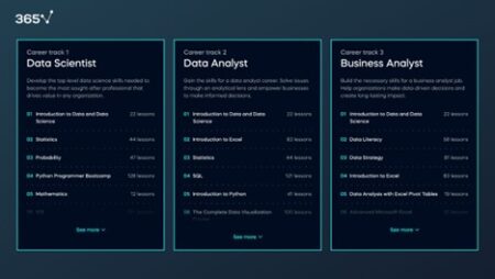
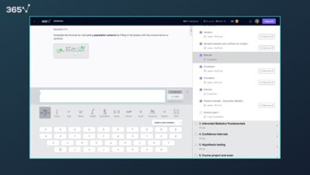
With over 2 million global users, 365 Data Science empowers learners with essential skills in data science, analytics, programming, and machine and deep learning. The e-learning platform provides a theoretical foundation for all data-related disciplines – Probability, Statistics, and Mathematics. 365’s curriculum also offers a comprehensive introduction to R programming, statistics in R, and courses on data visualization in R.

Tradition & Mission: Enduring Endeavors

Currently in its third season, the 365 Data Science annual free access initiative—born during the initial COVID-19 lockdown—relaunches. CEO Ned Krastev defines data science as “an ever-evolving field offering immense opportunities for career advancement,” underscoring the company’s dedication to nurturing a global network of maturing data talents and avid learners.

The initiative’s impact is impressive, with over 152,000 unique users from 200 countries in 2022 alone, accessing more than 9.2 million minutes of content and earning 38,761 certificates. Krastev marvels at the yearly growth in student engagement, attributing it to their zeal for learning and excelling in new roles. He reaffirms 365 Data Science’s unwavering commitment to supporting these learners on their path to success.

New Features & Learning Insights

365 has launched a collection of real-world, data-focused projects for various skill levels and technical requirements. Users can solve authentic business cases to acquire practical skills, boosting their employability and portfolio. Ned states, “Our focus on practice-based learning is crucial for skill mastery. We’re dedicated to equipping students with pertinent skills from the beginning, and we’re excited to see how these projects will advance their careers.”

Join the program and start for free at  365 Data Science