slickR

We are happy to bring the slick JavaScript library to R. It is self-described as “the last carousel you’ll ever need”. This carousel is based on putting the elements of the carousel in a div HTML tag. This makes the carousel very versatile in what can be placed inside. Regular objects that are placed in a carousel can be for example: images, plots, tables, gifs, videos, iframes and even htmlwidgets.

  This tool helps review multiple outputs in an efficient manner and saves much needed space in documents and Shiny applications, while creating a user friendly experience. These carousels can be used directly from the R console, from RStudio, in Shiny apps and R Markdown documents.

Installation

CRAN
install.packages('slickR')
Github (dev)
devtools::install_github('metrumresearchgroup/slickR')

Examples

There are many options within the slick carousel, to get started with the basics we will show a few examples in the rest of the post. If you want to try out any of the examples you can go to this site where they are rendered and can be tested out.

library(svglite)
library(lattice)
library(ggplot2)
library(rvest) 
library(reshape2)
library(dplyr)
library(htmlwidgets)
library(slickR)

Images

Some web scraping for the images example….
#NBA Team Logos
nbaTeams=c("ATL","BOS","BKN","CHA","CHI","CLE","DAL","DEN","DET","GSW",
    "HOU","IND","LAC","LAL","MEM","MIA","MIL","MIN","NOP","NYK",
    "OKC","ORL","PHI","PHX","POR","SAC","SAS","TOR","UTA","WAS")
teamImg=sprintf("https://i.cdn.turner.com/nba/nba/.element/img/4.0/global/logos/512x512/bg.white/svg/%s.svg",nbaTeams)

#Player Images
a1=read_html('http://www.espn.com/nba/depth')%>%html_nodes(css = '#my-teams-table a')
a2=a1%>%html_attr('href')
a3=a1%>%html_text()
team_table=read_html('http://www.espn.com/nba/depth')%>%html_table()
team_table=team_table[[1]][-c(1,2),]
playerTable=team_table%>%melt(,id='X1')%>%arrange(X1,variable)
playerName=a2[grepl('[0-9]',a2)]
playerId=do.call('rbind',lapply(strsplit(playerName,'[/]'),function(x) x[c(8,9)]))
playerId=playerId[playerId[,1]!='phi',]
playerTable$img=sprintf('http://a.espncdn.com/combiner/i?img=/i/headshots/nba/players/full/%s.png&w=350&h=254',playerId[,1])

Grouped Images

There are players on each team, so lets group the starting five together and have each dot correspond with a team:
slickR(
  obj = playerTable$img,
  slideId = c('ex2'),
  slickOpts = list(
    initialSlide = 0,
    slidesToShow = 5,
    slidesToScroll = 5,
    focusOnSelect = T,
    dots = T
  ),
  height = 100,width='100%'
)

Replacing the dots

Sometimes the dots won’t be informative enough so we can switch them with an HTML object, such as text or other images. We can pass to the customPaging argument javascript code using the htmlwidgets::JS function.

Replace dots with text

cP1=JS("function(slick,index) {return '<a>'+(index+1)+'</a>';}")

slickR(
  obj = playerTable$img,
  slideId = 'ex3',
  dotObj = teamImg,
  slickOpts = list(
    initialSlide = 0,
    slidesToShow = 5,
    slidesToScroll = 5,
    focusOnSelect = T,
    dots = T,
    customPaging = cP1
  ),
  height=100,width='100%'
)

Replace dots with Images

cP2=JS("function(slick,index) {return '<a><img src= ' + dotObj[index] + '  width=100% height=100%></a>';}")


#Replace dots with Images
s1 <- slickR(
  obj = playerTable$img,
  dotObj = teamImg,
  slickOpts = list(
    initialSlide = 0,
    slidesToShow = 5,
    slidesToScroll = 5,
    focusOnSelect = T,
    dots = T,
    customPaging = cP2
  ),height = 100,width='100%'
)

#Putting it all together in one slickR call
s2 <- htmltools::tags$script(
  sprintf("var dotObj = %s", 
          jsonlite::toJSON(teamImg))
)

htmltools::browsable(htmltools::tagList(s2, s1))

Plots

To place plots directly into slickR we use svglite to convert a plot into svg code using xmlSVG and then convert it into a character object
plotsToSVG=list(
  #Standard Plot
    xmlSVG({plot(1:10)},standalone=TRUE),
  #lattice xyplot
    xmlSVG({print(xyplot(x~x,data.frame(x=1:10),type="l"))},standalone=TRUE),
  #ggplot
    xmlSVG({show(ggplot(iris,aes(x=Sepal.Length,y=Sepal.Width,colour=Species))+
                   geom_point())},standalone=TRUE), 
  #lattice dotplot
    xmlSVG({print(dotplot(variety ~ yield | site , data = barley, groups = year,
                          key = simpleKey(levels(barley$year), space = "right"),
                          xlab = "Barley Yield (bushels/acre) ",
                          aspect=0.5, layout = c(1,6), ylab=NULL))
            },standalone=TRUE) 
)

#make the plot self contained SVG to pass into slickR 
s.in=sapply(plotsToSVG,function(sv){paste0("data:image/svg+xml;utf8,",as.character(sv))})
slickR(s.in,slideId = 'ex4',slickOpts = list(dots=T), height = 200,width = '100%')

Synching Carousels

There are instances when you have many outputs at once and do not want to go through all, so you can combine two carousels one for viewing and one for searching.
slickR(rep(s.in,each=5),slideId = c('ex5up','ex5down'),
       slideIdx = list(1:20,1:20),
       synchSlides = c('ex5up','ex5down'),
       slideType = rep('img',4),
       slickOpts = list(list(slidesToShow=1,slidesToScroll=1),
                        list(dots=F,slidesToScroll=1,slidesToShow=5,
                             centerMode=T,focusOnSelect=T)
                        ),
       height=100,width = '100%'
       )

Iframes

Since the carousel can accept any html element we can place iframes in the carousel. There are times when you may want to put in different DOMs rather than an image in slick. Using slideType you can specify which DOM is used in the slides. For example let’s put the help Rd files from ggplot2 into a slider using the helper function getHelp. (Dont forget to open the output to a browser to view the iframe contents).
geom_filenames=ls("package:ggplot2",pattern = '^geom')

slickR(unlist(lapply(geom_filenames,getHelp,pkg = 'ggplot2')),slideId = 'ex6',slideType = 'iframe',height = '400px',width='100%',slickOpts = list(dots=T,slidesToShow=2,slidesToScroll=2))

htmlwidgets

Finally, we can really leverage R and place self contained htmlwidgets in iframes (like leaflets and plotly) and use them in a carousel. This solves a problem of how to run many htmlwidgets at once outside of Shiny.
library(leaflet)
library(plotly)

l <- leaflet() %>% addTiles()
htmlwidgets::saveWidget(l,'leaflet.html')

p <- iris%>%ggplot(aes(x=Sepal.Length,y=Sepal.Width))+geom_point()
pL= ggplotly(p)
htmlwidgets::saveWidget(pL,'ggplotly.html')

slickR(c(rep(paste0(readLines('leaflet.html'),collapse='\n'),4),
         rep(paste0(readLines('ggplotly.html'),collapse='\n'),4)),
       slideId = c('leaf','plot'),
       slideIdx = list(1:4,5:8),
       slideType = rep('iframe',2),
       slickOpts = list(list(dots=T,slidesToShow=2,slidesToScroll=2),
                        list(dots=T,slidesToShow=2,slidesToScroll=2)),
       height='200px',width='100%')

Jonathan Sidi joined Metrum Research Group in 2016 after working for several years on problems in applied statistics, financial stress testing and economic forecasting in both industrial and academic settings. To learn more about additional open-source software packages developed by Metrum Research Group please visit the Metrum website. Contact: For questions and comments, feel free to email me at: [email protected] or open an issue for bug fixes or enhancements at github.

R Function Call with Ellipsis Trap/Pitfall

Objective if this post: alerting all users to double check case and spelling of all function parameters

I am newbie in R and was trying RSNNS mlp function and wasted a lot of time due to some typos.

RSNNS mlp function silently ignores misspelled keywords
Example:
model&lt;-mlp(iris[,1:4],decodeClassLabels(iris[,5]),hize=7,mazit=100)
I intentionally misspelled size as hize and maxit as mazit
There are no warnings or errors.

I think that many packages may have same problem as package writers may not always validate ellipsis arguments. I made a small spelling mistake and got puzzling results as there was no parameter validation, but I expected that great eminent packages should be robust and help users recover from typos Let us see what happens with no ellipsis
&gt; square &lt;-function(num ){
+ return(num*num)
+ }
&gt; 
&gt; square(num=4)
[1] 16
&gt; square(numm=4)
Error in square(numm = 4) : unused argument (numm = 4)

# With ellipsis added
&gt; square &lt;-function(num, …){
+ print(names(list(…)));
+ return(num*num)
+ }
&gt; 
&gt; square(num=3,bla=4,kla=9)
[1] “bla” “kla”
[1] 9
As you can see names(list(…)) does give access to parameter names The problem is that ellipsis function calls are for flexibility but package writers should take extra care to throw exception “unused argument” when parameters of functions are misspelled.

This to my mind is a major weakness of the R ecosystem. Most parameters have defaults and small case or spelling mistake can lead to really wrong conclusions!

RSNNS  is simply fantastic but given simply as an example of the ellipsis function call trap. Hope other newbies benefit and learn to avoid the trap of wrong arguments.

Jayanta Narayan Choudhuri
Kolkata India

ggedit 0.2.0 is now on CRAN

Jonathan Sidi, Metrum Research Group

ggedit 
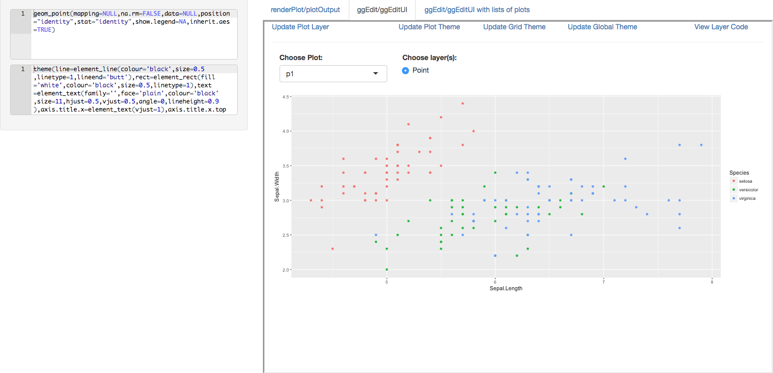
We are pleased to announce the release of the ggedit package on CRAN. To install the package you can call the standard R command
install.packages('ggedit')
The source version is still tracked on github, which has been reorganized to be easier to navigate. To install the dev version:
devtools::install_github('metrumresearchgroup/ggedit')

What is ggedit?

ggedit is an R package that is used to facilitate ggplot formatting. With ggedit, R users of all experience levels can easily move from creating ggplots to refining aesthetic details, all while maintaining portability for further reproducible research and collaboration. ggedit is run from an R console or as a reactive object in any Shiny application. The user inputs a ggplot object or a list of objects. The application populates Bootstrap modals with all of the elements found in each layer, scale, and theme of the ggplot objects. The user can then edit these elements and interact with the plot as changes occur. During editing, a comparison of the script is logged, which can be directly copied and shared. The application output is a nested list containing the edited layers, scales, and themes in both object and script form, so you can apply the edited objects independent of the original plot using regular ggplot2 grammar. Why does it matter? ggedit promotes efficient collaboration. You can share your plots with team members to make formatting changes, and they can then send any objects they’ve edited back to you for implementation. No more email chains to change a circle to a triangle!

Updates in ggedit 0.2.0:

  • The layer modal (popups) elements have been reorganized for less clutter and easier navigation.
  • The S3 method written to plot and compare themes has been removed from the package, but can still be found on the repo, see plot.theme.

Deploying

  • call from the console: ggedit(p)
  • call from the addin toolbar: highlight script of a plot object on the source editor window of RStudio and run from toolbar.
  • call as part of Shiny: use the Shiny module syntax to call the ggEdit UI elements.
    • server: callModule(ggEdit,'pUI',obj=reactive(p))
    • ui: ggEditUI('pUI')
  • if you have installed the package you can see an example of a Shiny app by executing runApp(system.file('examples/shinyModule.R',package = 'ggedit'))

Outputs

ggedit returns a list containing 8 elements either to the global enviroment or as a reactive output in Shiny.
  • updatedPlots
    • List containing updated ggplot objects
  • updatedLayers
    • For each plot a list of updated layers (ggproto) objects
    • Portable object
  • updatedLayersElements
    • For each plot a list elements and their values in each layer
    • Can be used to update the new values in the original code
  • updatedLayerCalls
    • For each plot a list of scripts that can be run directly from the console to create a layer
  • updatedThemes
    • For each plot a list of updated theme objects
    • Portable object
    • If the user doesn’t edit the theme updatedThemes will not be returned
  • updatedThemeCalls
    • For each plot a list of scripts that can be run directly from the console to create a theme
  • updatedScales
    • For each plot a list of updated scales (ggproto) objects
    • Portable object
  • updatedScaleCalls
    • For each plot a list of scripts that can be run directly from the console to create a scale
 

Short Clip to use ggedit in Shiny


Jonathan Sidi joined Metrum Research Group in 2016 after working for several years on problems in applied statistics, financial stress testing and economic forecasting in both industrial and academic settings. To learn more about additional open-source software packages developed by Metrum Research Group please visit the Metrum website. Contact: For questions and comments, feel free to email me at: [email protected] or open an issue for bug fixes or enhancements at github.

Web data acquisition: parsing json objects with tidyjson (Part 3)

The collection of example flight data in json format available in part 2, described the libraries and the structure of the POST request necessary to collect data in a json object. Despite the process generated and transferred locally a proper response, the data collected were neither in a suitable structure for data analysis nor immediately readable. They appears as just a long string of information nested and separated according to the JavaScript object notation syntax. Thus, to visualize the deeply nested json object and make it human readable and understandable for further processing, the json content could be copied and pasted in a common online parser. The tool allows to select each node of the tree and observe the data structure up to the variables and data of interest for the statistical analysis. The bulk of the relevant information for the purpose of the analysis on flight prices are hidden in the tripOption node as shown in the following figure (only 50 flight solutions were requested). 
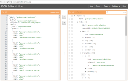
However, looking deeply into the object, several other elements are provided as the distance in mile, the segment, the duration, the carrier, etc. The R parser to transform the json structure in a usable dataframe requires the dplyr library for using the pipe operator (%>%) to streamline the code and make the parser more readable. Nevertheless, the library actually wrangling through the lines is tidyjson and its powerful functions:
  • enter_object: enters and dives into a data object;
  • gather_array: stacks a JSON array;
  • spread_values: creates new columns from values assigning specific type (e.g. jstring, jnumber).
library(dplyr) # for pipe operator %>% and other dplyr functions library(tidyjson) # https://cran.r-project.org/web/packages/tidyjson/vignettes/introduction-to-tidyjson.html data_items <- datajson %>% spread_values(kind = jstring("kind")) %>% spread_values(trips.kind = jstring("trips","kind")) %>% spread_values(trips.rid = jstring("trips","requestId")) %>% enter_object("trips","tripOption") %>% gather_array %>% spread_values( id = jstring("id"), saleTotal = jstring("saleTotal")) %>% enter_object("slice") %>% gather_array %>% spread_values(slice.kind = jstring("kind")) %>% spread_values(slice.duration = jstring("duration")) %>% enter_object("segment") %>% gather_array %>% spread_values( segment.kind = jstring("kind"), segment.duration = jnumber("duration"), segment.id = jstring("id"), segment.cabin = jstring("cabin")) %>% enter_object("leg") %>% gather_array %>% spread_values( segment.leg.aircraft = jstring("aircraft"), segment.leg.origin = jstring("origin"), segment.leg.destination = jstring("destination"), segment.leg.mileage = jnumber("mileage")) %>% select(kind, trips.kind, trips.rid, saleTotal,id, slice.kind, slice.duration, segment.kind, segment.duration, segment.id, segment.cabin, segment.leg.aircraft, segment.leg.origin, segment.leg.destination, segment.leg.mileage) head(data_items) kind trips.kind trips.rid saleTotal 1 qpxExpress#tripsSearch qpxexpress#tripOptions UnxCOx4nKIcIOpRiG0QBOe EUR178.38 2 qpxExpress#tripsSearch qpxexpress#tripOptions UnxCOx4nKIcIOpRiG0QBOe EUR178.38 3 qpxExpress#tripsSearch qpxexpress#tripOptions UnxCOx4nKIcIOpRiG0QBOe EUR235.20 4 qpxExpress#tripsSearch qpxexpress#tripOptions UnxCOx4nKIcIOpRiG0QBOe EUR235.20 5 qpxExpress#tripsSearch qpxexpress#tripOptions UnxCOx4nKIcIOpRiG0QBOe EUR248.60 6 qpxExpress#tripsSearch qpxexpress#tripOptions UnxCOx4nKIcIOpRiG0QBOe EUR248.60 id slice.kind slice.duration 1 ftm7QA6APQTQ4YVjeHrxLI006 qpxexpress#sliceInfo 510 2 ftm7QA6APQTQ4YVjeHrxLI006 qpxexpress#sliceInfo 510 3 ftm7QA6APQTQ4YVjeHrxLI009 qpxexpress#sliceInfo 490 4 ftm7QA6APQTQ4YVjeHrxLI009 qpxexpress#sliceInfo 490 5 ftm7QA6APQTQ4YVjeHrxLI007 qpxexpress#sliceInfo 355 6 ftm7QA6APQTQ4YVjeHrxLI007 qpxexpress#sliceInfo 355 segment.kind segment.duration segment.id segment.cabin 1 qpxexpress#segmentInfo 160 GixYrGFgbbe34NsI COACH 2 qpxexpress#segmentInfo 235 Gj1XVe-oYbTCLT5V COACH 3 qpxexpress#segmentInfo 190 Grt369Z0shJhZOUX COACH 4 qpxexpress#segmentInfo 155 GRvrptyoeTfrSqg8 COACH 5 qpxexpress#segmentInfo 100 GXzd3e5z7g-5CCjJ COACH 6 qpxexpress#segmentInfo 105 G8axcks1R8zJWKrN COACH segment.leg.aircraft segment.leg.origin segment.leg.destination segment.leg.mileage 1 320 FCO IST 859 2 77W IST LHR 1561 3 73H FCO ARN 1256 4 73G ARN LHR 908 5 319 FCO STR 497 6 319 STR LHR 469 Data are now in an R-friendly structure despite not yet ready for analysis. As can be observed from the first rows, each record has information on a single segment of the flight selected. A further step of aggregation using some SQL is needed in order to end up with a dataframe of flights data suitable for statistical analysis. Next up, the aggregation, some data analysis and data visualization to complete the journey through the web data acquisition using R. #R #rstats #maRche #json #curl #tidyjson #Rbloggers This post is also shared in www.r-bloggers.com and LinkedIn

Web data acquisition: the structure of RCurl request (Part 2)

The acquisition of data in json structure presented in part 1 clearly showed the functioning of the client-server connection and the possibility to collect the data of interest. However, the json output appeares as a set of raw data in a json string that needs to be structured and stored in a suitable form for data processing and statistical analysis.

For this reason, it makes sense to develop the entire process using #R in order to have the data directly queried, collected, parsed, structured and made usable in a unique environment. Of course, this will be the one used in the process “last mile”, i.e. data analysis. The curl library adopted in the command line process described in the previous post has its alter ego in the RCurl library. Together with jsonlite for ‘R-JSON translation’ these are the necessay packages for the development of the request as presented in the following code. [splus] # before loading the libraries rememeber to install them – install.packages(‘library here’) library(RCurl) library(jsonlite) # save the url of the request in an object (same as -X POST in the curl request) url <- ‘https://www.googleapis.com/qpxExpress/v1/trips/search?key={SERVER_KEY}&alt=json’ # headers (same as -H) headers <- list(‘Accept’ = ‘application/json’, ‘Content-Type’ = ‘application/json’, ‘charset’ = ‘UTF-8’) # R structure of the input for the request (same as -d + JSON) x = list( request = list( slice = list( list(origin = ‘FCO’, destination = ‘LHR’, date = ‘2017-06-30’)), passengers = list(adultCount = 1, infantInLapCount = 0, infantInSeatCount = 0, childCount = 0, seniorCount = 0), solutions = 500, refundable = F)) # url, headers and x are the parameters to be used in R functions to send the request # and save the output data in the datajson object # postForm is the RCurl function to send the request using the POST method # toJSON is the jsonlite function to convert the R structure of the request in JSON input datajson <- postForm(url, .opts=list(postfields=toJSON(x), httpheader=headers)) datajson [/splus] After few seconds from the POST request necessary to send the request and collect the response, all the information related to the flights with origin FCO (Fiumicino – Rome) and destination LHR (London Heathrow) will be hosted in the datajson object, similarly to the command line procedure. The json string holds and hides all the observations and variables of interest for the statistical analysis inlcuding the most important, i.e. the flight prices. The next post will explain how to parse the json object and structure the information in a suitable dataframe for analysis using the powerful library #tidyjson. #R #rstats #maRche #json #curl #qpxexpress #Rbloggers This post is also shared in www.r-bloggers.com and LinkedIn

Web data acquisition: understanding RCurl from the command line (Part 1)

After the short presentation here, let’s start using R seriously, i.e. with every day data.

Being a frequent flyer, I often search the web to book flights and organise my trip. Being a data analyst, it’s natural to look at price data with interest, especially the most convenient, most expensive and “average” flights. Being a PhD student in software engineering the (study) programme includes some on the structure of applications, client-server data flows and the web languages running the processes. Nothing like Google flight API QPX express would have been better to combine all these three. I discovered it by chance delving into the first results of my flight searches on Google and it is perfect for some web scraping and analysis. As described in the manual, QPX Express is part of the Google suite of publicly-available REST APIs, designed for easy integration, fast response and high reliability. QPX Express searches combinations of airline schedules, fares and seat availability and includes search parameters such as origin, destination, dates and travel features such as maximum price and earliest departure. The API returns up to 500 itineraries for each request, including all data elements needed for customer display and a booking process. Moreover, it also allows to clearly see the structure of the data in #json both in input (JSON request) and output (Unformatted Response). For a simple test, use the Demo with a Google account. Before start using the QPX Express API, you need to get a Google API key. To get a key, follow these steps: 1. Go to the Google Developers Console / 2. Create or select a project / 3. Click Continue to enable the API and any related services / 4. On the Credentials page, get an API key. With a single API key, it is possible to make 50 free requests per day (then the cost per single query is $ 0.035.) The first thing I tried before writing the code in #R for data acquisition, manipulation and analysis was to test the client-server connection through a command line instruction using the cURL library (you can download here – add the certificate in the same directory otherwise the server will deny you access). Let’s play a bit with the command line (Windows 10) before running the request:
# open the command prompt and the default folder should be system32 of the OS
C:\WINDOWS\system32>

# set a convenient current directory (cd) for storing data - \ (enter) and / (exit) the path
cd C:\Users\Roberto\Desktop

# your new position should be in 
C:\Users\Roberto\Desktop>


# I prefer using a partition of the HD dedicated to data instead of a messy desktop
cd /D D:\

# create a new working directory (use "" for separated names otherwise two folders will be created)
mkdir "flight data"
# set the current directory to the newly created folder
cd "flight data"
# make sub-folders of the cd
mkdir "curl test 1"
mkdir "curl test 2"
# check the cd, its features and its new sub-folders
cd

dir

# finally, check the proper installation of curl using help
# the list of the function parameters should appear with some description

curl -help
After the creation of a repository, cURL can be used for testing the connection to QPX express and the collection of data in json using cURL parameters for HTTP requests and the structure of the JSON request the API proposes:
# Parameters
# -X POST: parameter for POST request -> see: https://en.wikipedia.org/wiki/POST_(HTTP)
# -H: Pass custom header LINE to server (H) -> see: https://en.wikipedia.org/wiki/List_of_HTTP_header_fields
# -d: HTTP POST data, i.e. the input data in JSON structure 
# >: "send to" destination file

curl -X POST "https://www.googleapis.com/qpxExpress/v1/trips/search?key={SERVER_KEY}&alt=json" -H "Content-Type: application/json; charset=UTF-8" -d "{ \"request\": { \"slice\": [ { \"origin\": \"{ORIGIN_CODE}\", \"destination\": \"{DESTINATION_CODE}\", \"date\": \"{DATE_YYYY-MM-DD}\" } ], \"passengers\": { \"adultCount\": 1, \"infantInLapCount\": 0, \"infantInSeatCount\": 0, \"childCount\": 0, \"seniorCount\": 0 }, \"solutions\": 500, \"refundable\": false }}" > "{RESULT_FILE}.json"
# Mac syntax
curl -X POST 'https://www.googleapis.com/qpxExpress/v1/trips/search?key={SERVER_KEY}&alt=json' -H 'Content-Type: application/json; charset=UTF-8' -d '{ "request": { "slice": [ { "origin": "{ORIGIN_CODE}", "destination": "{DESTINATION_CODE}", "date": "{DATE_YYYY-MM-DD}" } ], "passengers": { "adultCount": 1, "infantInLapCount": 0, "infantInSeatCount": 0, "childCount": 0, "seniorCount": 0 }, "solutions": 500, "refundable": false }}'> '{RESULT_FILE}.json'
After a second, the prompt should show the downloading process stats and a new json file should appear in the cd “flight data” close to the previously created subfolders. The connection works! Next up – a post with code to translate the same commands in R – to manipulate the data comfortably after acquisition from the API. #R #rstats #maRche #json #curl #qpxexpress #Rbloggers This post is also shared in www.r-bloggers.com and LinkedIn

ggedit 0.1.1: Shiny module to interactvely edit ggplots within Shiny applications

ggedit is a package that lets users interactively edit ggplot layer and theme aesthetics. In a previous post we showed you how to use it in a collaborative workflow using standard R scripts. More importantly, we highlighted that ggedit outputs to the user, after editing, updated: gg plots, layers, scales and themes as both self-contained objects and script that you can paste directly in your code.

Installation

devtools::install_github('metrumresearchgroup/ggedit',subdir='ggedit')

version 0.1.1 Updates

  • ggEdit Shiny module: use ggedit as part of any Shiny application.
  • gggsave: generalized ggsave to write multiple outputs of ggplot to a single file and/or multiple files from a single call. Plots can be saved to various graphic devices. 

ggEdit Shiny module

This post will demonstrate a new method to use ggedit, Shiny modules. A Shiny module is a chunk of Shiny code that can be reused many times in the same application, but generic enough so it can be applied in any Shiny app (in simplest terms think of it as a Shiny function). By making ggedit a Shiny module we can now replace any renderPlot() call that inputs a ggplot and outputs in the UI plotOutput(), with an interactive ggedit layout. The analogy between how to use the ggEdit module in comparison to a standard renderPlot call can be seen in the table below.
  Standard Shiny Shiny Module
Server output$id=renderPlot(p) reactiveOutput=callModule(ggEdit,id,reactive(p))
UI plotOutput(id) ggEditUI(id)
We can see that there are a few differences in the calls. To call a module you need to run a Shiny function callModule, in this case ggEdit. Next, a character id for the elements the module will create in the Shiny environment and finally the arguments that are expected by the module, in this case a reactive object that outputs a ggplot or list of ggplots. This is coupled with ggEditUI, which together create a ggedit environment to edit the plots during a regular Shiny app. In addition to the output UI the user also gets a reactive output that has all the objects that are in the regular ggedit package (plots, layers, scales, themes) both in object and script forms. This has great advantages if you want to let users edit plots while keeping track of what they are changing. A realistic example of this would be clients (be it industry or academia) that are shown a set of default plots, with the appropriate data, and then they are given the opportunity to customize according to their specifications. Once they finish editing, the script is automatically saved to the server, updating the clients portfolio with their preferred aesthetics. No more email chains on changing a blue point to an aqua star! Below is a small example of a static ggplot using renderPlot/plotOutput and how to call the same plot and a list of plots using ggEdit/ggeditUI. We added a small reactive text output so you can see the real-time changes of the aesthetic editing being returned to the server [youtube https://www.youtube.com/watch?v=pJ1kbd_OVwg]

Source Code for example

library(ggedit)
server = function(input, output,session) {
p1=ggplot(iris,aes(x=Sepal.Length,y=Sepal.Width,colour=Species))+geom_point()
p2=ggplot(iris,aes(x=Sepal.Length,y=Sepal.Width,colour=Species))+geom_line()+geom_point()
p3=list(p1=p1,p2=p2)
output$p=renderPlot({p1})

outp1=callModule(ggEdit,'pOut1',obj=reactive(list(p1=p1)))
outp2=callModule(ggEdit,'pOut2',obj=reactive(p3))

output$x1=renderUI({
layerTxt=outp1()$UpdatedLayerCalls$p1[[1]]
aceEditor(outputId = 'layerAce',value=layerTxt,
mode = 'r', theme = 'chrome',
height = '100px', fontSize = 12,wordWrap = T)
})

output$x2=renderUI({
themeTxt=outp1()$UpdatedThemeCalls$p1
aceEditor(outputId = 'themeAce',value=themeTxt,
mode = 'r', theme = 'chrome',
height = '100px', fontSize = 12,wordWrap = T)
})
}

ui=fluidPage(
conditionalPanel("input.tbPanel=='tab2'",
sidebarPanel(uiOutput('x1'),uiOutput('x2'))),
mainPanel(
tabsetPanel(id = 'tbPanel',
tabPanel('renderPlot/plotOutput',value = 'tab1',plotOutput('p')),
tabPanel('ggEdit/ggEditUI',value = 'tab2',ggEditUI('pOut1')),
tabPanel('ggEdit/ggEditUI with lists of plots',value = 'tab3',ggEditUI('pOut2'))
)))
shinyApp(ui, server)

gggedit

ggsave is the device writing function written for the ggplot2 package. A limitation of it is that only one figure can be written at a time. gggsave is a wrapper of ggsave that allows for list of ggplots to be called and then passes arguments to base graphics devices to create multiple outputs automatically, without the need of loops.
library(ggedit) 
#single file output to pdf 
gggsave('Rplots.pdf',plot=pList) 

#multiple file output to pdf 
gggsave('Rplots.pdf',plot=pList,onefil = FALSE) 

#multiple file output to png 
gggsave('Rplots.png',plot=pList)


Jonathan Sidi joined Metrum Research Group in 2016 after working for several years on problems in applied statistics, financial stress testing and economic forecasting in both industrial and academic settings.


To learn more about additional open-source software packages developed by Metrum Research Group please visit the Metrum website.


Contact: For questions and comments, feel free to email me at: [email protected] or open an issue in github.