So you want to learn Shiny? Congratulations, great decision!
Shiny is a wonderful tool for creating web applications using just R – without JavaScript, ASP.NET, Ruby on Rails or other programming languages. And the output is absolutely remarkable – beautiful charts, tables and text that present information in a highly attractive way.
Learning Shiny is not terribly hard, even if you are an absolute beginner. You just need some proper guidance. This is why I have created this tutorial that drives you through the process of creating a simple Shiny application, from A to Z.
It’s a long tutorial, so make sure you’re sitting in a comfortable chair and have pen and paper at hand, to take notes. If you want to follow along and code with me in RStudio, that’s even better.
Let’s dive straight in.
What Are We Going to Build?
Let’s start with the end in sight – let’s see first how our app is going to look like. Click below link (opens in a new window) and take a minute to play around with the app, then come back here. I’ll be waiting for you.
https://bestshiny.shinyapps.io/income/
Back already? OK, let’s go on…
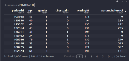
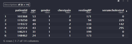
The data set used to build this app is called demographics and contains information about 510 customers of a big company. The variables of interest for us are age, gender and income. You can see a fragment of the data set in the image below.
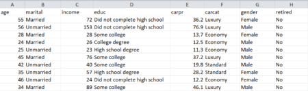
To download the entire data file, click here:
http://www.shiny-academy.com/downloads/demographics.csv
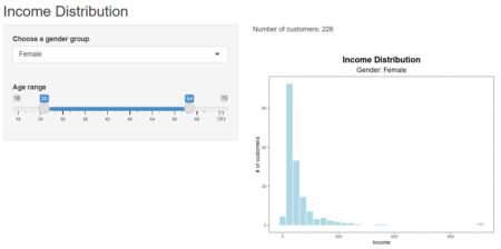
When the user selects a gender category and an age range, the app displays the following outputs:
- the number of customers that meet the specified criteria
- a histogram that presents the income distribution for those customers
As you could notice, this information updates instantly any time the user modifies their selection.
So let’s build this app from scratch. However, before even writing the first line of code we must become familiar with the basic components of any Shiny app.
Let’s Understand the Shiny App Structure
Every app is made up of two parts: user interface and server.
The user interface (or, briefly, UI) is actually a web page that the app user sees. As you know, the language of the web pages is HTML. Therefore, the user interface is HTML code that we write using different Shiny functions.
The Shiny app interface contains:
-
- the inputs that allow the user to interact with the app
- the outputs generated by the app in different formats (text, tables, charts, images etc.)
Let’s look at our app, for example.
Its interface has four elements:
-
- two input objects: a dropdown menu and a slider
- two output objects: a text block and a chart
So, the user interface creates the whole application layout – it indicates the exact place and configuration of each element in the page.
The second component of a Shiny app is the server.
The role of the server is to create the outputs (text, tables, charts etc.) using a set of instructions. These instructions are actually R functions and commands. So the Shiny server recognises any code that can be run by the R program.
Your Shiny server can operate:
-
- on a local computer, i.e. your own computer (when you run the app in RStudio)
- on a remote computer (a server located in another place)
As you remember, the outputs of our app update automatically when you change the input values. Why is that? What happens, actually?
Whenever an input is modified, the server re-creates the outputs using the instructions that we have written. This mechanism is called reactivity, and it’s the essential attribute of any Shiny application.
So far, so good. Now that we know the components of a Shiny application, we can write the skeleton of our own app.
The Essential App Template
All Shiny apps have the same basic template, presented in the picture below.
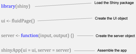
As you notice, this basic template has four lines.
In the first line we load the Shiny package using the library function. That’s self explanatory.
In the second line we create the user interface object, called ui. To build the ui object we use the fluidPage function. As the name shows, this function produces a fluid web page, i.e. a web page with flexible layout. More precisely, the elements in the page are resized in real time so they fit in the browser window.
All the objects in the user interface (inputs and outputs) will be written inside this function.
The third line initialises the server object, the second component of the application. This object is called server.
The server object is created using an R function. This function has two arguments: input and output. So the server function takes the input values (specified by the user) and creates the output objects that will be displayed in the user interface.
The fourth line is very important, because here we call a function that assembles our app: shinyApp. When the program notices this function, it recognises our file as being a Shiny application.
The shinyApp function has two arguments that correspond to the core components of our app: ui and server. As you can see, the ui argument takes the value “ui”, because this is the name of the user interface object. The server argument takes the value “server”, because server is the name of our server object. So this function tells the program which is which:
-
- which is the user interface (in our case, ui) and
- which is the server (in our case, server)
Very important: this line must be the last line of code in your app. So don’t write anything below it. Please keep this in mind.
Before running a Shiny app you must save it under a name (it is advisable to save it in a separate folder, where you don’t have any other apps or R scripts). Then you press the “Run App” button at the top of the editor.
Adding Some Formatting
OK, now we know the basic structure of a Shiny app. It’s time to build a neat interface layout.
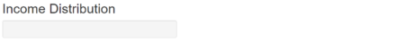
If you look at our app interface, the first thing you probably notice is the big heading (“Income Distribution”). To create a heading we can use the titlePanel function. We are going to write this function inside the fluidPage function, because the heading is an element of the user interface. Our app code will look like this:
library(shiny)

ui <- fluidPage (

titlePanel("Income Distribution")

)

server <- function (input, output) {}

shinyApp(ui = ui, server = server)
Furthermore, you can see that the input objects are placed in a side area at left, while the output elements are displayed in the central area. This type of arrangement is called “sidebar layout”, and is created with a special function called, well… sidebarLayout. In the sidebar layout we define two areas:
-
- the left panel, using the sidebarPanel function
- the main area, using the mainPanel function
Obviously, all these functions must be written inside the user interface object (i.e. inside the fluidPage function). Let’s add them to our code:
library(shiny)

ui <- fluidPage (

titlePanel("Income Distribution"),

sidebarPanel(

),

mainPanel(

)

)

server <- function (input, output) {}

shinyApp(ui = ui, server = server)
There is something very important in the code above that you must notice: I have put a comma after titlePanel and another comma after sidebarPanel. So in your code you must separate all the elements in the user interface by commas. It’s an essential rule that you should always remember. If you forget the commas, your app will crash.
When you run the code above, you see the following:
So all we have in our interface right now is the title. It’s time to create the other components. However, there are a couple of things to do before that.
First Things First
In the beginning, we have to load the needed packages. Our app uses two R packages: dplyr (for data manipulation) and ggplot2 (to draw the chart). So we must add two lines of code just before the ui object:
library(shiny)

library(dplyr)

library(ggplot2)

ui <- fluidPage (

titlePanel("Income Distribution"),

sidebarPanel(

),

mainPanel(

)

)

server <- function (input, output) {}

shinyApp(ui = ui, server = server)
Next, we have to load our working data set, using the read.csv command. I am going to call my data set object demo. Please make sure that the CSV file (your data source) is placed in the same folder with the app.
Let’s write a new line of code to load the data set:
library(shiny)

library(dplyr)

library(ggplot2)

demo <- read.csv("demographics.csv", stringsAsFactors = FALSE)

ui <- fluidPage (

titlePanel("Income Distribution"),

sidebarPanel(

),

mainPanel(

)

)

server <- function (input, output) {}

shinyApp(ui = ui, server = server)
Great. Now that we got this out of the way, let’s take care of the user interface objects.
Building the Inputs
We can create many types of input controls in Shiny, using particular input functions. For this app we only need two inputs: a dropdown menu and a slider.
Any input control in Shiny has two main parameters:
-
- a name or id. This id must be unique. Please make sure that you don’t have two input objects with the same id in your app.
- a label or description. This label is optional, but useful. Your app users cannot see the input id, but they can see the label.
Besides id and label, each input control has its own specific parameters.
Now let’s write the functions that create our input controls.
To generate a dropdown menu we use the selectInput function. We’ll write this function inside the sidebarPanel function (because the input controls are located in the sidebar area). Please take a look at the code below to see the arguments of the selectInput function:
library(shiny)

library(dplyr)

library(ggplot2)

demo <- read.csv("demographics.csv", stringsAsFactors = FALSE)

ui <- fluidPage (

titlePanel("Income Distribution"),

sidebarPanel(

selectInput("gender", "Choose a gender group", choices = c("Female", "Male"))

),

mainPanel(

)

)

server <- function (input, output) {}

shinyApp(ui = ui, server = server)
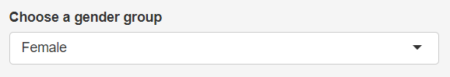
So our input is called “gender” and its label is “Choose a gender group”. The menu options (male and female) are introduced with the choices argument. The first option in the list is selected by default. Our dropdown menu looks like this:
Everything’s fine, so let’s get to the second input object.
To create a slider control we use the sliderInput function. Just like any other input, a slider has an id and a label. In addition, we must define the following parameters:
-
- the slider limits (lower and upper)
- the selected value(s). Our slider must allow us to define a range of values (for the age variable), so we must specify two default selected values (minimum and maximum).
Let’s write the sliderInput function now. First we have to put a comma after selectInput (as you remember, the objects in the user interface must be separated by commas). Then we write our function as you can see below:
library(shiny)

library(dplyr)

library(ggplot2)

demo <- read.csv("demographics.csv", stringsAsFactors = FALSE)

ui <- fluidPage (

titlePanel("Income Distribution"),

sidebarPanel(

selectInput("gender", "Choose a gender group", choices = c("Female", "Male")),

sliderInput("age", "Age range", min = 18, max = 73, value = c(25, 45))

),

mainPanel(

)

)

server <- function (input, output) {}

shinyApp(ui = ui, server = server)
Our slider id is “age”, and its label is “Age range”. The lower and upper limits are 18 and 73, respectively (these are the minimum and maximum age values in our data set). As for the default age range, it is defined as being 25-45, using the value argument. The slider object looks like this:
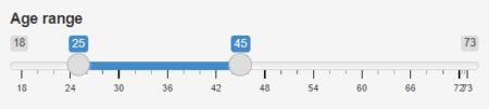
You notice that it has two handles that let the user specify an age interval between the minimum and the maximum age values.
OK, we are done with the inputs. Are you still with me? Excellent! Let’s move on to the output elements.
Creating the Output Placeholders
Now we must tell the program what type of output objects we need and where to put them in the user interface. For this purpose we use the output placeholders.
The Shiny package provides different output functions, corresponding to different output categories. The argument of each output function is the output name (or id). This name must be written between double quotes.
Please note that these functions do not build output objects. They only create placeholders that indicate the outputs type and place. To actually generate the outputs we have to use server functions, as we’ll see a bit later.
As you know, our app has two output objects: a text output and a chart output. Both are placed in the main area of the interface, so we write them inside the mainPanel function.
To create a text output placeholder we use the textOutput function (easy to remember, right?). Let’s call our output “count”, for example (because it prints the number of customers). Writing it is very simple:
library(shiny)

library(dplyr)

library(ggplot2)

demo <- read.csv("demographics.csv", stringsAsFactors = FALSE)

ui <- fluidPage (

titlePanel("Income Distribution"),

sidebarPanel(

selectInput("gender", "Choose a gender group", choices = c("Female", "Male")),

sliderInput("age", "Age range", min = 18, max = 73, value = c(25, 45))

),

mainPanel(

textOutput("count")

)

)

server <- function (input, output) {}

shinyApp(ui = ui, server = server)
To build a plot placeholder we have to use the plotOutput function. The id of this output will be “chart”, for instance. So I will add another line to of code to my script:
library(shiny)

library(dplyr)

library(ggplot2)

demo <- read.csv("demographics.csv", stringsAsFactors = FALSE)

ui <- fluidPage (

titlePanel("Income Distribution"),

sidebarPanel(

selectInput("gender", "Choose a gender group", choices = c("Female", "Male")),

sliderInput("age", "Age range", min = 18, max = 73, value = c(25, 45))

),


mainPanel(

textOutput("count"),

br(),

plotOutput("chart")

)

)

server <- function (input, output) {}

shinyApp(ui = ui, server = server)
Please notice one more thing: between the placeholder functions I have written another function, br. This function inserts a line break between the objects. I did that to separate the visual elements with white space and avoid the sensation of clutter in the user interface. (Of course, you can put line breaks between the input objects as well.)
That’s all for it. Now the program knows which types of output we need and where they will be located.
Our user interface is ready: we have created both input controls and output placeholders. In the following sections we’ll move our focus to the server function, because it’s the server side of our app that actually builds the output objects.
What Will the Server Do?
Basically, the server part of our app has to perform the following operations:
-
- filter the data set applying the user’s selections
- print the output text (“count”)
- build the plot (“chart”)
These operations will be done with ordinary R code. However, I have a very important point to bring up here.
Our code will operate with reactive objects: Shiny inputs and outputs. These objects can only be handled in a particular type of environment called reactive environment or reactive context. So we must create this reactive context using a special Shiny function.
Now, before writing the code in the server part we have to understand how Shiny creates output objects.
Creating Output Objects
The Shiny program builds output objects using a three-step procedure.
First, it takes the necessary input values from the inputs list. You remember that the server function has an input argument, do you? Well, this argument is nothing but a list that contains all the input values. These values are accessed using the $ sign, just as we do with any list in R.
In our particular case we have three input values:
1. the gender category (male or female). To get this category we simply write:
input$gender
2. the minimum age. To get this age we must write:
input$age[1]
So the minimum value in a slider input takes the index 1.
3. the maximum age. To access this age we write:
input$age[2]
Yes, you guessed right: the maximum value in a slider input takes the index 2.
In the second step, the outputs are generated using a special rendering function. We’ll talk about these functions in a few moments.
Finally, in the third step, the outputs are saved in the outputs list. As you remember, the second argument of the server function is output. This argument is actually a list that contains all the output objects. To access any output we use the $ sign.
Our app has two output placeholders: a text placeholder called “count” and a plot placeholder called “chart”. Correspondingly, we are going to build two output objects – a text and a plot – that we’ll save with the same names in the outputs list. To access these objects we will write:
output$count
and
output$chart
It’s important to remember: the outputs must be saved with the same name as the corresponding placeholders, so the program can match them up. That should go without saying.
As soon as the outputs are saved, the placeholders are “filled” and the output objects are displayed in the user interface.
Let’s see how to complete these steps in practice, using our app example.
First Job: Filter the Data Set
Before everything, we must filter our data set. We are going to use the filter command in dplyr. Let’s take a look at the code:
library(shiny)

library(dplyr)

library(ggplot2)

demo <- read.csv("demographics.csv", stringsAsFactors = FALSE)

ui <- fluidPage (

titlePanel("Income Distribution"),

sidebarPanel(

selectInput("gender", "Choose a gender group", choices = c("Female", "Male")),

sliderInput("age", "Age range", min = 18, max = 73, value = c(25, 45))

),


mainPanel(

textOutput("count"),

br(),

plotOutput("chart")

)

)

server <- function (input, output) {

demo_filtered % filter(gender == input$gender,
                                      age >= input$age[1],
                                      age <= input$age[2])

})

}

shinyApp(ui = ui, server = server)
The filtering conditions are straightforward. The gender variable must be equal to the selected gender, and the age must be within the selected age range. But there is a key detail that I want you to notice: the filter command is placed inside another function called reactive. The role of this function is to create reactive context.
As I have explained above, we need this reactive context to handle the reactive variables used by the filter function (input$gender, input$age[1] and input$age[2]). If we try to work with reactive variables outside reactive context, our app crashes. This is an essential take away lesson.
We must call the reactive function using parentheses and curly brackets, as follows:
reactive({ })
The filtering result is stored in a new data set called demo_filtered. This data set is also a reactive object, because it was created with the reactive function. This is another important fact to keep in mind: all the objects created inside reactive context are reactive objects.
Furthermore, when we call a reactive object we must always put a pair of round brackets (parentheses) after it, just like this:
demo_filtered()
If you forget the parentheses, the app will not work. That’s because reactive objects are assimilated to functions, and R functions are always called using round brackets, as you know.
Fine. Now we have to count the number of entries in the filtered data set (because we must print this number in the user interface, right?). We are going to use another dplyr function, count. Let’s examine the code:
library(shiny)

library(dplyr)

library(ggplot2)

demo <- read.csv("demographics.csv", stringsAsFactors = FALSE)

ui <- fluidPage (

titlePanel("Income Distribution"),

sidebarPanel(

selectInput("gender", "Choose a gender group", choices = c("Female", "Male")),

sliderInput("age", "Age range", min = 18, max = 73, value = c(25, 45))

),


mainPanel(

textOutput("count"),

br(),

plotOutput("chart")

)

)

server <- function (input, output) {

demo_filtered % filter(gender == input$gender,
                                      age >= input$age[1],
                                      age <= input$age[2])

})

entries % count()

})

}

shinyApp(ui = ui, server = server)
First, I followed the rule stated above and put parentheses after the data set name (demo_filtered). Then, I wrote the count command inside the reactive function. Why? Because demo_filtered is a reactive object, so it cannot be manipulated outside reactive context. So we absolutely need to create reactive context with this function.
As a result, the variable entries (the number of entries) is a reactive object as well, so we must use round brackets any time we call it. I hope you’re beginning to get the hang of it.
Let’s go on. Time to create the outputs now.
Next Job: Print the Text
As I said in a previous section, Shiny builds output objects using rendering functions. For the text outputs, this function is renderText. So any time we create a text placeholder with textOutput, we can “fill” that placeholder using renderText.
Let’s see how the code works:
library(shiny)

library(dplyr)

library(ggplot2)

demo <- read.csv("demographics.csv", stringsAsFactors = FALSE)

ui <- fluidPage (

titlePanel("Income Distribution"),

sidebarPanel(

selectInput("gender", "Choose a gender group", choices = c("Female", "Male")),

sliderInput("age", "Age range", min = 18, max = 73, value = c(25, 45))

),


mainPanel(

textOutput("count"),

br(),

plotOutput("chart")

)

)

server <- function (input, output) {

demo_filtered % filter(gender == input$gender,
                                      age >= input$age[1],
                                      age <= input$age[2])

})

entries % count()

})

output$count <- renderText({

paste0("Number of customers: ", entries())

})

}

shinyApp(ui = ui, server = server)
First, please note the syntax of renderText: it is called using rounded and curly brackets. This function produces reactive context, just like the reactive function, so it can work with reactive objects.
To create and print the text string we simply use the paste0 function from base R. Nothing special here. Please also note the parentheses after the variable entries (which is a reactive object).
In the end, we save our text as an object in the outputs list, under the name “count” (the corresponding placeholder name).
Now our text is shown in the main panel. Any time the user makes a new selection, the text changes accordingly (because the value of the variable entries changes).
Final Job: Plot the Chart
The function used to produce charts in Shiny is renderPlot. We need this function any time we have to “fill” a chart placeholder created with plotOutput.
The renderPlot function generates reactive context, so it can handle reactive variables. Inside it we can use any R function that creates charts; in our app we are going to use ggplot.
Let’s write the code now:
library(shiny)

library(dplyr)

library(ggplot2)

demo <- read.csv("demographics.csv", stringsAsFactors = FALSE)

ui <- fluidPage (

titlePanel("Income Distribution"),

sidebarPanel(

selectInput("gender", "Choose a gender group", choices = c("Female", "Male")),

sliderInput("age", "Age range", min = 18, max = 73, value = c(25, 45))

),


mainPanel(

textOutput("count"),

br(),

plotOutput("chart")

)

)

server <- function (input, output) {

demo_filtered % filter(gender == input$gender,
                                      age >= input$age[1],
                                      age <= input$age[2])

})

entries % count()

})

output$count <- renderText({

paste0("Number of customers: ", entries())

})

output$chart <- renderPlot(

width = 500,

height = 400,

{

ggplot(demo_filtered(), aes(income))+
                         geom_histogram(fill = "lightblue",      color="white")+
                         xlab("Income")+
                         ylab("# of customers")+
                         theme(panel.background = element_rect(fill = "white",
                         colour = "black"))+
                         labs(title = "Income Distribution",
                         subtitle = paste0("Gender: ", input$gender))+
                         theme(plot.title = element_text(size = 17, hjust = 0.5, face = "bold"),
                         plot.subtitle = element_text(size = 14, hjust = 0.5))


})

}

shinyApp(ui = ui, server = server)
So, the chart data source is demo_filtered (called with round brackets, because it’s a reactive object) and the chart is drawn with geom_histogram. The subtitle is created dynamically: it changes when the gender group changes (to accomplish that, we inserted the input$gender variable in the subtitle argument, as you can see).
Please notice one more thing: the width and height parameters (chart dimensions) are set in the beginning, before opening the curly brackets.
The rest of the code is usual ggplot code, so I’m not going to comment it.
Finally, we save our plot in the outputs list, under the name “chart” – the same name as the corresponding placeholder. At this moment, our chart is displayed in the user interface.
Well, it’s over now. Our app is done and functional.
Congratulations, great work! You have just created your first Shiny application starting from zero.
Isn’t There More to Shiny Than This?
Yes. A lot more.
Shiny can build sophisticated applications that use advanced data analysis and machine learning models. It can create dynamic input controls and complex, good-looking user interfaces that use HTML and CSS. It can draw interactive charts, work with files (for example, upload a data set from disk and use it further) and much more.
If you want to learn how to build similar apps (and many more), I highly recommend the free chapter of my new Shiny video course. Actually, it’s a two-hour mini-course that introduces the basics of Shiny. If you like what you see there, you can get the whole course.
Click here to start learning Shiny for free


 The mean and the standard error of the sample is close to the population mean and standard deviation.
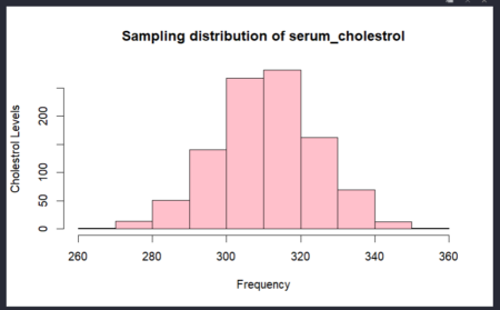

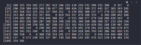
 The mean of the sample 2 with sample size 200 is 308.875 .