Hi fellow R users (and Qualtrics users),
As many Qualtrics surveys produce really similar output datasets, I created a tutorial with the most common steps to clean and filter data from datasets directly downloaded from Qualtrics.
You will also find some useful codes to handle data such as creating new variables in the dataframe from existing variables with functions and logical operators.
The tutorial is presented in the format of a downloadable R code with explanations and annotations of each step. You will also find a raw Qualtrics dataset to work with.
Link to the tutorial: https://github.com/angelajw/QualtricsDataCleaning
This dataset comes from a Qualtrics survey with an experiment format (control and treatment conditions), but the codes can be applicable to non-experimental datasets as well, as many cleaning steps are the same.
Category: R
New Version of the Package “Vecsets” is on CRAN
The
For this revision, the code for most functions was rewritten to increase processing speed dramatically. A new function, “vperm,” generates all permutations of all possible combinations taken N elements at a time from an input vector.
base “sets” tools follow the algebraic definition that each element of a set must be unique. Since it’s often helpful to compare all elements of two vectors, this toolset treats every element as unique for counting purposes. For ease of use, all functions in vecsets have an argument multiple which, when set to FALSE , reverts them to the base set tools functionality.For this revision, the code for most functions was rewritten to increase processing speed dramatically. A new function, “vperm,” generates all permutations of all possible combinations taken N elements at a time from an input vector.
Hackathon sponsored by NanoString Technologies
NanoString Technologies is sponsoring a hackathon with DevPost to spur development of tools and methods in the form of R packages for its GeoMx Spatial Biology platform. GeoMx allows measurement of protein and RNA expression within selected regions of a tissue slide versus having to measure the slide as a whole. This allows you to compare expression between tumor and non-tumor cells within a tumor biopsy slide, for example.
A dataset from a collection of kidney biopsy samples is available for use in the hackathon and packages that either create new and insightful graphs or data analysis methods are encouraged. NanoString has developed some infrastructure packages based on ExpressionSets that are available on Bioconductor to allow developers to focus more on graphs and methods versus data input.
A top prize of $10,000 is available to the top winner with other prizes for second and third place winners. Details can be found at the hackathon website.
https://nanostring.devpost.com/
#rstats
ExpDes: An R Package for ANOVA
Analysis of variance (ANOVA) is an usual way for analysing experiments. However, depending on the design and/or the analysis scheme, it can be a hard task. ExpDes, acronym for Experimental Designs, is a package that intends to turn such task easier. Devoted to fixed models and balanced experiments, ExpDes allows the user to deal with additional treatments in a single run, several experiment designs and exhibits standard and easy-to-interpret outputs.
[contact-form][contact-field label=”Name” type=”name” required=”true” /][contact-field label=”Email” type=”email” required=”true” /][contact-field label=”Website” type=”url” /][contact-field label=”Message” type=”textarea” /][/contact-form]
The main purpose of the package ExpDes is to analyze simple experiments under completely randomized designs (crd()), randomized block designs (cbd()) and Latin square designs (latsd()). Also enables the analysis of treatments in a factorial design with 2 and 3 factors (fat2.crd(), fat3.crd(), fat2.rbd(), fat3.rbd()) and also the analysis of split-plot designs (split2.crd(), split2.rbd()). Other functionality is analyzing experiments with one additional treatments on completely randomized design and randomized blocks design with 2 or 3 factors (fat2.ad.crd(), fat2.ad.rbd(), fat3.ad.crd() and fat3.ad.crd()).
After loading the package and reading and attaching the data, a single command is required to analyze any situation. For instance, consider a completely randomized design for a qualitative factor.
crd(treat, resp, quali = TRUE, mcomp = "tukey")
crd(trat, resp, quali = FALSE, sigF = 0.05)
---------------------------------------------------------------
Analysis of Variance Table
---------------------------------------------------------------
DF SS MS Fc Pr>Fc
Treatament 3 214.88 71.626 6.5212 0.0029622
Residuals 20 219.67 10.984
Total 23 434.55
---------------------------------------------------------------
CV = 3.41 %
---------------------------------------------------------------
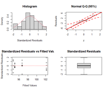
Shapiro-Wilk normality test
p-value: 0.91697
According to Shapiro-Wilk normality test at 5% of significance,
residuals can be considered normal.
---------------------------------------------------------------
---------------------------------------------------------------
Homogeneity of variances test
p-value: 0.1863216
According to the test of bartlett at 5% of significance,
residuals can be considered homocedastic.
---------------------------------------------------------------
Tukey's test
---------------------------------------------------------------
Groups Treatments Means
a A 102.1983
b B 96.74333
b C 95.05833
b D 94.74333
---------------------------------------------------------------
 a <- crd(treat, resp)
 plotres(a)
[contact-form][contact-field label=”Name” type=”name” required=”true” /][contact-field label=”Email” type=”email” required=”true” /][contact-field label=”Website” type=”url” /][contact-field label=”Message” type=”textarea” /][/contact-form]
From “Sh*t’s Creek” to “Schitt’s Creek”: On Padding Surnames with Extra Letters
We typically think of English and related spelling systems as mapping orthographic units or graphemes onto units of speech sounds, or phonemes. For instance, each of the three letters in “pen” maps to the three phonemes /p/, /ɛ/, and /n/ in the spoken version of the word. But there is considerable flexibility in the English spelling system, enabling other information to be encoded while still preserving phonemic mapping. For example, padding the ends of disyllabic words with extra unpronounced letters indicates that accent or stress should be placed on the second syllabic instead of the more common English pattern of first syllable stress(e.g., compare “trusty” with “trustee”, “gravel” with “gazelle”, or “rivet” with “roulette).
Proper names provide a rich resource for exploring how spelling systems are used to convey more than sound. Consider “Gerry” and “Gerrie” for example. These names are pronounced the same, but the final vowel /i/ is spelled differently. The difference is associated with gender: Between 1880 and 2016, 99% of children named “Gerrie” have been girls compared with 32% of children named “Gerry.” More generally, as documented in the code below, name-final “ie” is more associated with girls than boys. On average, names ending in “ie” and “y” are given to girls 84% and 66% of the time respectively (i.e., names ending in the sound /i/ tend to be given to girls, but more so if spelled with “ie” than “y”).
I tested this hypothesis using a data set of surnames occurring at least 100 times in the 2010 US Census. Specifically, I flagged all monosyllabic names that ended in double letters. I restricted to monosyllabic names since letter doubling can affect accent placement, as noted above, which could create differences between the padded and unpadded versions. Next, I stripped off the final letter from these names and matched to a sentiment dictionary. Finally, I tested whether surnames were more likely to be padded if the unpadded version expressed negative sentiment.
The following R code walks through these steps. We’ll start by first reading the downloaded csv file of surnames into a data frame, and then converting the surnames from upper case in the Census file to lower case for mapping to a sentiment dictionary:
Next, we’ll flag all monosyllabic names using the nsyllable function in the Quanteda package, identify those with a final double letter, and place into a new data frame:
Finally, we’ll create a variable that strips each name of its final letter (e.g., “grimm” becomes “grim”) and match the latter to a sentiment dictionary, VADER (“Valence Aware Dictionary for sEntiment Reasoning”) specifically. We’ll then put the matching words into a new data frame:
The final set of surnames is small – just 36 cases after removing one duplicate. It’s a small enough dataset to list them all:
An alternative explanation for this pattern is that there are more surnames with negative than positive sentiment overall, providing greater opportunity for negative surnames to be padded with extra letters. However, if anything, there are slightly more surnames with positive than negative sentiment in the Census database (294 vs. 254).
In sum, US surnames are more likely to be padded with extra letters when the unpadded version would express negative rather than positive sentiment. These results align with other naming patterns that indicate an aversion toward negative sentiment. Such aversions are consistent with nominal realism or the cross-cultural tendency to transfer connotations from a name to the named.
Finally, in case you’re wondering, no—“Schitt,” “Shitt,” nor “Sh*t” appear in the US Census database of surnames (at least in 2010). However, “Dicke,” “Asse,” and “Paine” do appear, illustrating another way to pad proper names besides letter doubling: Adding a final unpronounced “e.” But that’s a tale for another blog….
Proper names provide a rich resource for exploring how spelling systems are used to convey more than sound. Consider “Gerry” and “Gerrie” for example. These names are pronounced the same, but the final vowel /i/ is spelled differently. The difference is associated with gender: Between 1880 and 2016, 99% of children named “Gerrie” have been girls compared with 32% of children named “Gerry.” More generally, as documented in the code below, name-final “ie” is more associated with girls than boys. On average, names ending in “ie” and “y” are given to girls 84% and 66% of the time respectively (i.e., names ending in the sound /i/ tend to be given to girls, but more so if spelled with “ie” than “y”).
#Data frame I created from US Census dataset of baby names
load("/Users/MHK/R/Baby Names/NamesOverall.RData")
sumNames$final_y_ie <- grepl("y$|ie$",sumNames$Name)
final_y_ie <- filter(sumNames, final_y_ie==TRUE)
final_y_ie$prop_f <- final_y_ie$femaleTotal/final_y_ie$allTotal
t.test(final_y_ie$prop_f[grepl("ie$",final_y_ie$Name)],final_y_ie$prop_f[grepl("y$",final_y_ie$Name)])
    Welch Two Sample t-test

t = 20.624, df = 7024.5, p-value < 2.2e-16
alternative hypothesis: true difference in means is not equal to 0
95 percent confidence interval:
 0.1684361 0.2038195
sample estimates:
mean of x mean of y
0.8412466 0.6551188
Capitalizing the first letter in proper nouns is perhaps the most well-known example of how we use the flexibility in spelling systems to convey information beyond pronunciation. More subtly, we sometimes increase the prominence of proper names by padding with extra unpronounced letters as in “Penn” versus “pen” and “Kidd” versus “kid.” An interesting question is what factors influence whether or not a name is padded. Which brings us to Schitt’s Creek. The title of the popular series plays exactly on the fact that padding the name with extra letters that don’t affect pronunciation hides the expletive. This suggests a hypothesis: Padded names should be more common when the unpadded version contains negative sentiment, which might carry over via psychological “contagion” from the surname to the person. So, surnames like “Grimm” and “Sadd” should be more common than surnames like “Winn.”I tested this hypothesis using a data set of surnames occurring at least 100 times in the 2010 US Census. Specifically, I flagged all monosyllabic names that ended in double letters. I restricted to monosyllabic names since letter doubling can affect accent placement, as noted above, which could create differences between the padded and unpadded versions. Next, I stripped off the final letter from these names and matched to a sentiment dictionary. Finally, I tested whether surnames were more likely to be padded if the unpadded version expressed negative sentiment.
The following R code walks through these steps. We’ll start by first reading the downloaded csv file of surnames into a data frame, and then converting the surnames from upper case in the Census file to lower case for mapping to a sentiment dictionary:
library(tidyverse)
surnames <- read.csv("/Users/mike/R/Names/Names_2010Census.csv",header=TRUE)
surnames$name <- tolower(surnames$name)
Next, we’ll flag all monosyllabic names using the nsyllable function in the Quanteda package, identify those with a final double letter, and place into a new data frame:
Library(quanteda)
surnames$num_syllables <- nsyllable(surnames$name)
surnames$finalDouble <- grepl("(.)\\1$", surnames$name)
oneSylFinalDouble <- filter(surnames, num_syllables == 1 & finalDouble == TRUE)
oneSylFinalDouble <- select(oneSylFinalDouble, name, num_syllables, finalDouble)
Finally, we’ll create a variable that strips each name of its final letter (e.g., “grimm” becomes “grim”) and match the latter to a sentiment dictionary, VADER (“Valence Aware Dictionary for sEntiment Reasoning”) specifically. We’ll then put the matching words into a new data frame:
oneSylFinalDouble$Stripped <- substr(oneSylFinalDouble$name,1,nchar(oneSylFinalDouble$name)-1)
vader <- read.csv("/Users/MHK/R/Lexicon/vader_sentiment_words.csv",header=TRUE)
vader$word <- as.character(vader$word)
vader <- select(vader,word,mean_sent)
oneSylFinalDouble <- left_join(oneSylFinalDouble, vader, by=c("Stripped"="word"))
sentDouble <- filter(oneSylFinalDouble, !(is.na(mean_sent)))
The final set of surnames is small – just 36 cases after removing one duplicate. It’s a small enough dataset to list them all:
select(sentDouble,name, mean_sent) %>% arrange(mean_sent)
      name mean_sent
1     warr      -2.9
2   cruell      -2.8
3    stabb      -2.8
4    grimm      -2.7
5     robb      -2.6
6     sinn      -2.6
7     bann      -2.6
8  threatt      -2.4
9    hurtt      -2.4
10  grieff      -2.2
11    fagg      -2.1
12    sadd      -2.1
13   glumm      -2.1
14   liess      -1.8
15   crapp      -1.6
16    nagg      -1.5
17    gunn      -1.4
18   trapp      -1.3
19   stopp      -1.2
20   dropp      -1.1
21    cutt      -1.1
22   dragg      -0.9
23    rigg      -0.5
24    wagg      -0.2
25  stoutt       0.7
26    topp       0.8
27    fann       1.3
28    fitt       1.5
29  smartt       1.7
30    yess       1.7
31   gladd       2.0
32    hugg       2.1
33    funn       2.3
34    wonn       2.7
35    winn       2.8
36    loll       2.9
Of these 36 cases, 24 have negative sentiment when the final letter is removed and only 12 positive sentiment, a significant skew toward padding surnames that would express negative sentiment if unpadded as determined through a one-tailed binomial test:binom.test(24,36, alternative=c("greater"))
Exact binomial test
data: 24 and 36
number of successes = 24, number of trials = 36, p-value = 0.03262
alternative hypothesis: true probability of success is greater than 0.5
95 percent confidence interval:
0.516585 1.000000
sample estimates:
probability of success
0.6666667
An alternative explanation for this pattern is that there are more surnames with negative than positive sentiment overall, providing greater opportunity for negative surnames to be padded with extra letters. However, if anything, there are slightly more surnames with positive than negative sentiment in the Census database (294 vs. 254).
In sum, US surnames are more likely to be padded with extra letters when the unpadded version would express negative rather than positive sentiment. These results align with other naming patterns that indicate an aversion toward negative sentiment. Such aversions are consistent with nominal realism or the cross-cultural tendency to transfer connotations from a name to the named.
Finally, in case you’re wondering, no—“Schitt,” “Shitt,” nor “Sh*t” appear in the US Census database of surnames (at least in 2010). However, “Dicke,” “Asse,” and “Paine” do appear, illustrating another way to pad proper names besides letter doubling: Adding a final unpronounced “e.” But that’s a tale for another blog….
Sentiment Analysis of Surnames
Sentiment analysis is typically applied to connected text such as product reviews. However, it can also be extended to names, potentially delivering rich insights into psychology and culture. Globally and historically, names hold important familial, cultural, and religious significance. The foundation for much of this significance is a concept called nominal realism, which holds that the name imbues characteristics into the named. For instance, personal names in many cultures are based on totemic animals so that valued traits of the totem are transferred to the human namesake. We see nominal realism in our own culture from our tendency to name sports teams such as the Detroit Lions and Chicago Bears after predatory animals with stereotypically aggressive dispositions rather than, say, the Cincinnati Sloths, Chicago Sheep, or Green Bay Guinea Pigs.
My own research has examined nominal realism in names by documenting biases toward positive versus negative sentiment in names. For example, in cultures around the world, people emphasize the positive more than the negative in everyday speech. But I found a much more pronounced focus on the positive in a sentiment analysis of US place names. The positivity bias is especially large in names of cities and towns – which are closely connected to the self – than names of natural features. More recently, I’ve shown that business names also show a strong bias toward positive over negative words – with consequences for business performance. Specifically, revenues of businesses containing negative words are significantly lower than those for businesses containing positive or neutral words.
In this post, I will extend sentiment analysis to surnames such as “Smith” and “Jones”. Surnames are interesting since technically they have no meaning, although they may at one time. Today’s “Shoemakers” for example are probably no more likely to be in that profession than those with other surnames (though I suppose this is an assumption that warrants testing). That said, sentiment analysis would code surnames like “Grief” and “Coward” as negative while “Hardy” and “Courage” would be coded positive. Nominal realism would predict that negative surnames would be less common than positive surnames given fears that negative characteristics of the name would carry over to the named.
I tested this hypothesis using a data set of surnames occurring at least 100 times in the 2010 US Census. We’ll start the analysis by first reading the downloaded csv file into a data frame, and then streamlining to just the two key variables used in the analysis, the name and count of occurrences:
surnames <- read.csv("/Users/mike/R/Names/Names_2010Census.csv",header=TRUE)
surnames <- select(surnames, name, count)
head(surnames)
      name   count
1    SMITH 2442977
2  JOHNSON 1932812
3 WILLIAMS 1625252
4    BROWN 1437026
5    JONES 1425470
6   GARCIA 1166120
Next, we’ll convert the surnames to lower case for matching to a sentiment dictionary:
surnames$name <- tolower(surnames$name)We’ll identify surnames with positive or negative sentiment using the AFINN sentiment lexicon, specifically the 2011 version. Each of the 2477 words in this lexicon is coded with an integer score ranging from -5 to +5 with negative/positive values reflecting sentiment valence and magnitude. I downloaded this lexicon, saving in Excel which we’ll load and merge with the surnames data frame. We’ll then remove all non-matching surnames (i.e., the vast majority of names like “Baker” and “Smith” with neutral sentiment).
affin <- read_excel("/Users/mike/R/AFFIN_Sentiment_Lexicon.xlsx", sheet="AFINN-111")
surnames <- left_join(surnames,affin,by=c("name"="Word"))
surname_sent <- filter(surnames,!is.na(Sentiment))
This leaves us with 332 surnames with a coded sentiment score, representing 13% of the words in the AFINN sentiment lexicon. We can look at a few surnames randomly selected from those with positive and negative sentiment to get a sense for them:
filter(surname_sent, Sentiment > 0) %>% slice_sample(n=10)
        name count Sentiment
1       free  9923         1
2      mercy   575         2
3    freedom   138         2
4       gift  1490         2
5   straight  4307         1
6       fair 18609         2
7      spark   472         1
8     heaven   625         2
9      hardy 80252         2
10 brilliant   491         4

filter(surname_sent, Sentiment < 0) %>% slice_sample(n=10)
      name count Sentiment
1     fail   754        -2
2  failing   717        -2
3   sullen   401        -2
4    angry   154        -3
5     bias  6518        -1
6     sore   115        -1
7    moody 64429        -1
8    blind   835        -1
9     glum   118        -2
10    lack  2661        -2
Next, we’ll test whether surnames with positive sentiment occur more frequently than those with negative sentiment, as nominal realism would predict. Consistent with other word frequency analyses that include words with a huge frequency range (100-2,442,977), we’ll first convert the frequency counts to logs and use those values in a t-test:
t.test(log10(surname_sent$count[surname_sent$Sentiment >0]),log10(surname_sent$count[surname_sent$Sentiment < 0]))
    Welch Two Sample t-test

data:  log10(surname_sent$count[surname_sent$Sentiment > 0]) and log10(surname_sent$count[surname_sent$Sentiment < 0])
t = 3.5516, df = 322.6, p-value = 0.0004399
alternative hypothesis: true difference in means is not equal to 0
95 percent confidence interval:
 0.1283081 0.4469758
sample estimates:
mean of x mean of y
 3.130305  2.842663
Results were in the predicted direction, with mean frequency of positive surnames ~1350 and negative surnames ~700, or almost 2:1.
I replicated the results using another sentiment lexicon.
In sum, surname usage in the US shows a bias toward positive sentiment/avoidance of negative sentiment similar to those seen in US place and business names. It would be interesting to test whether there are significant consequences of having a negative surname (e.g., like the analysis of negative business names described above). New version of cgwtools package is up
I’m happy to present some info about the latest version of cgwtools, my collection of handy “toys” which make everyday work in R a bit easier. Enjoy!
The newly added functions include:
base2base – Function to convert any base to any other base (up to 36).
binit — Create histogram bins for each unique value in a sample. That is, automatically use the unique values as bin ranges, rather than dividing up the overall range by some factor.
cumfun — Function calculate the cumulative result of any function along an input vector.
maxn , minn — Functions to find the n-th maximum or minimum of a vector or array.
which.maxn , which.minn — Functions to find locations of the n-th maximum or minimum of a vector or array.
polyInt — Function to find intersection points of two polygons.
segSegInt — Function to find intersection point between two line segments (NOT lines).
Other functions previously provided:
approxeq — Do “fuzzy” equality and return a logical vector (rather than a single status as all.equal does).
dim — Function to return dimensions of arguments, or lengths if dim==NULL.
findpat — Function to locate patterns ( sequences of strings or numerical values) in data vectors.
popd , pushd — Performs equivalent of ‘bash’ command with same name
getstack — Returns the current directory stack that pushd and popd manipulate
dirdir — Wrapper function around dir() which returns only directories found in the specified location(s).
lsclass, lssize, lstype — list all objects with the specified class, size, type .
lsdata — List all objects in an ‘.Rdata’ file.
maxRow, maxCol, minRow, MinCol — Functions which mimic ‘max.col’ to find minimum or maximum of rows or columns.
mystat — Calculate and display basic statistics (max, min, mean, median, std dev, skew, kurtosis) for an object.
resave — Add some objects to an existing ‘.Rdata’ – type file.
seqle — Extends ‘rle’ to find and encode linear sequences.
inverse.seqle — Inverse of ‘seqle’
ease_aes() Demo
Easing
In R, easing is the interpolation, or tweening, between successive states of a plot (1). It is used to control the motion of data elements in animated data displays (2), with different easing functions giving different appearances or dynamics to the display’s animation.The ease_aes() Function
The ease_aes() function controls the easing of aesthetics or variables in gganimate. The default, ease_aes(), models a linear transition between states. Other easing functions are specified using the easing function name, appended with one of three modifiers (3) :Easing Functions
quadratic models an exponential function of exponent 2.cubic models an exponential function of exponent 3.
quartic models an exponential function of exponent 4.
quintic models an exponential function of exponent 5.
sine models a sine function.
circular models a pi/2 circle arc.
exponential models an exponential function of base 2.
elastic models an elastic release of energy.
back models a pullback and release.
bounce models the bouncing of a ball.
Modifiers
-in applies the easing function as-is.-out applies the easing function in reverse.
-in-out applies the first half of the transition as-is and the last half in reverse.
The formulas used to implement these options can be found here (4). They are illustrated below using animated scatter plots and bar charts.
Data File Description
‘data.frame’: 40 obs. of 7 variables:Cat : chr “A” “A” “A” “A” …
OrdInt: int 1 2 3 4 5 1 2 3 4 5 …
X : num 70.5 78.1 70.2 78.1 70.5 30.7 6.9 26.7 6.9 30.7 …
Y : num 1.4 7.6 -7.9 7.6 1.4 -7 -23.8 19.8 -23.8 -7 …
Rank : int 2 2 2 2 2 7 8 8 8 7 …
OrdDat: chr “01/01/2019” “04/01/2019” “02/01/2019” “05/01/2019” …
Ord : Date, format: “2019-01-01” “2019-04-01” “2019-02-01” “2019-05-01” …
The data used for this demo is a much abbreviated and genericized version of this (5) data set.
Scatter Plots
Here is the code used for the ease_aes(‘cubic-in’) animated scatter plot:# load libraries
library(gganimate)
library(tidyverse)
# the data file format is indicated above
data <- read.csv('Data.csv')
# convert date to proper format
data$Ord <- as.Date(data$OrdDat, format='%m/%d/%Y')
# specify the animation length and rate
options(gganimate.nframes = 30)
options(gganimate.fps = 10)
# loop the animation
options(gganimate.end_pause = 0)
# specify the data source and the X and Y variables
ggplot(data, aes(X, Y)) +
# specify the plot format
theme(panel.background = element_rect(fill = 'white'))+
theme(axis.line = element_line()) +
theme(axis.text = element_blank())+
theme(axis.ticks = element_blank())+
theme(axis.title = element_blank()) +
theme(plot.title = element_text(size = 20)) +
theme(plot.margin = margin(25, 25, 25, 25)) +
theme(legend.position = 'none') +
# create a scatter plot
geom_point(aes(color = Cat), size = 5) +
# indicate the fill color scale
scale_fill_viridis_d(option = "D", begin = 0, end = 1) +
# apply the fill to the 'Cat' variable
aes(group = Cat) +
# animate the plot on the basis of the 'Ord' variable
transition_time(Ord) +
# the ease_aes() function
ease_aes('cubic-in') +
# title the plot
labs(title = "'ease_aes(cubic-in)'")
 |
 |
 |
 |
 |
 |
 |
 |
 |
 |
 |
 |
 |
 |
 |
 |
 |
 |
 |
 |
 |
 |
 |
 |
 |
 |
 |
 |
 |
 |
 |
Bar Charts
Here is the code used for the ease_aes(‘cubic-in’) animated bar chart:# load libraries library(gganimate) library(tidyverse) # the data file format is indicated above data <- read.csv('Data.csv') # convert date to proper format data$Ord <- as.Date(data$OrdDat, format='%m/%d/%Y') # specify the animation length and rate options(gganimate.nframes = 30) options(gganimate.fps = 10) # loop the animation options(gganimate.end_pause = 0) # specify the data source ggplot(data) + # specify the plot format theme(panel.background = element_rect(fill = 'white'))+ theme(panel.grid.major.x = element_line(color='gray'))+ theme(axis.text = element_blank())+ theme(axis.ticks = element_blank())+ theme(axis.title = element_blank()) + theme(plot.title = element_text(size = 20)) + theme(plot.margin = margin(25, 25, 25, 25)) + theme(legend.position = 'none') + # specify the x and y plot limits aes(xmin = 0, xmax=X+2) + aes(ymin = Rank-.45, ymax = Rank+.45, y = Rank) + # create a bar chart geom_rect() + # indicate the fill color scale scale_fill_viridis_d(option = "D", begin = 0, end = 1) + # place larger values at the top scale_y_reverse() + # apply the fill to the 'Cat' variable aes(fill = Cat) + # animate the plot on the basis of the 'Ord' variable transition_time(Ord) + # the ease_aes() function ease_aes('cubic-in') + # title the plot labs(title = "'ease_aes(cubic-in)'")
 |
 |
 |
 |
 |
 |
 |
 |
 |
 |
 |
 |
 |
 |
 |
 |
 |
 |
 |
 |
 |
 |
 |
 |
 |
 |
 |
 |
 |
 |
 |
Other Resources
Here (6) is a nice illustration of the various easing options presented as animated paths.Here (7) and here (8) are articles presenting various animated plots using ease_aes().
Here (9) are some other animations using ease_aes().
References
1 https://www.rdocumentation.org/packages/gganimate/versions/1.0.7/topics/ease_aes2 https://rdrr.io/cran/tweenr/
3 https://gganimate.com/reference/ease_aes.html
4 https://github.com/thomasp85/tweenr/blob/master/src/easing.c
5 https://academic.udayton.edu/kissock/http/Weather/default.htm
6 https://easings.net/
7 https://github.com/ropenscilabs/learngganimate/blob/master/ease_aes.md
8 https://www.statworx.com/de/blog/animated-plots-using-ggplot-and-gganimate/
9 https://www.r-graph-gallery.com/animation.html
Isovists using uniform ray casting in R
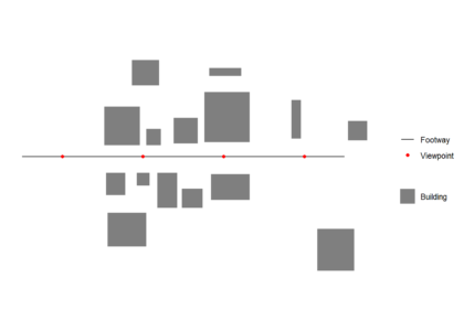
Isovists are polygons of visible areas from a point. They remove views that are blocked by objects, typically buildings. They can be used to understanding the existing impact of, or where to place urban design features that can change people’s behaviour (e.g. advertising boards, security cameras or trees). Here I present a custom function that creates a visibility polygon (isovist) using a uniform ray casting “physical” algorithm in R.
First we load the required packages (use
First we load the required packages (use
install.packages() first if these are not already installed in R):library(sf)
library(dplyr)
library(ggplot2)
Data generation
First we create and plot an example footway with viewpoints and set of buildings which block views. All data used should be in the same Coordinate Reference System (CRS). We generate one viewpoint every 50 m (note density here is a function of the st_crs() units, in this case meters)library(sf)
footway <- st_sfc(st_linestring(rbind(c(-50,0),c(150,0))))
st_crs(footway) = 3035
viewpoints <- st_line_sample(footway, density = 1/50)
viewpoints <- st_cast(viewpoints,"POINT")
buildings <- rbind(c(1,7,1),c(1,31,1),c(23,31,1),c(23,7,1),c(1,7,1),
c(2,-24,2),c(2,-10,2),c(14,-10,2),c(14,-24,2),c(2,-24,2),
c(21,-18,3),c(21,-10,3),c(29,-10,3),c(29,-18,3),c(21,-18,3),
c(27,7,4),c(27,17,4),c(36,17,4),c(36,7,4),c(27,7,4),
c(18,44,5), c(18,60,5),c(35,60,5),c(35,44,5),c(18,44,5),
c(49,-32,6),c(49,-20,6),c(62,-20,6),c(62,-32,6),c(49,-32,6),
c(34,-32,7),c(34,-10,7),c(46,-10,7),c(46,-32,7),c(34,-32,7),
c(63,9,8),c(63,40,8),c(91,40,8),c(91,9,8),c(63,9,8),
c(133,-71,9),c(133,-45,9),c(156,-45,9),c(156,-71,9),c(133,-71,9),
c(152,10,10),c(152,22,10),c(164,22,10),c(164,10,10),c(152,10,10),
c(44,8,11),c(44,24,11),c(59,24,11),c(59,8,11),c(44,8,11),
c(3,-56,12),c(3,-35,12),c(27,-35,12),c(27,-56,12),c(3,-56,12),
c(117,11,13),c(117,35,13),c(123,35,13),c(123,11,13),c(117,11,13),
c(66,50,14),c(66,55,14),c(86,55,14),c(86,50,14),c(66,50,14),
c(67,-27,15),c(67,-11,15),c(91,-11,15),c(91,-27,15),c(67,-27,15))
buildings <- lapply( split( buildings[,1:2], buildings[,3] ), matrix, ncol=2)
buildings <- lapply(X = 1:length(buildings), FUN = function(x) {
st_polygon(buildings[x])
})
buildings <- st_sfc(buildings)
st_crs(buildings) = 3035
# plot raw data
ggplot() +
geom_sf(data = buildings,colour = "transparent",aes(fill = 'Building')) +
geom_sf(data = footway, aes(color = 'Footway')) +
geom_sf(data = viewpoints, aes(color = 'Viewpoint')) +
scale_fill_manual(values = c("Building" = "grey50"),
guide = guide_legend(override.aes = list(linetype = c("blank"),
nshape = c(NA)))) +
scale_color_manual(values = c("Footway" = "black",
"Viewpoint" = "red",
"Visible area" = "red"),
labels = c("Footway", "Viewpoint","Visible area"))+
guides(color = guide_legend(
order = 1,
override.aes = list(
color = c("black","red"),
fill = c("transparent","transparent"),
linetype = c("solid","blank"),
shape = c(NA,16))))+
theme_minimal()+
coord_sf(datum = NA)+
theme(legend.title=element_blank())
Isovist function
Function inputs
Buildings should be cast to"POLYGON" if they are not already
buildings <- st_cast(buildings,"POLYGON")
Creating the function
A few parameters can be set before running the function.rayno is the number of observer view angles from the viewpoint. More rays are more precise, but decrease processing speed.raydist is the maximum view distance. The function takessfc_POLYGON type and sfc_POINT objects as inputs for buildings abd the viewpoint respectively.
If points have a variable view distance the function can be modified by creating a vector of view distance of length(viewpoints) here and then selecting raydist[x] in st_buffer below.
Each ray is intersected with building data within its raycast distance, creating one or more ray line segments. The ray line segment closest to the viewpoint is then extracted, and the furthest away vertex of this line segement is taken as a boundary vertex for the isovist. The boundary vertices are joined in a clockwise direction to create an isovist.st_isovist <- function(
buildings,
viewpoint,
# Defaults
rayno = 20,
raydist = 100) {
# Warning messages
if(!class(buildings)[1]=="sfc_POLYGON") stop('Buildings must be sfc_POLYGON')
if(!class(viewpoint)[1]=="sfc_POINT") stop('Viewpoint must be sf object')
rayends <- st_buffer(viewpoint,dist = raydist,nQuadSegs = (rayno-1)/4)
rayvertices <- st_cast(rayends,"POINT")
# Buildings in raydist
buildintersections <- st_intersects(buildings,rayends,sparse = FALSE)
# If no buildings block max view, return view
if (!TRUE %in% buildintersections){
isovist <- rayends
}
# Calculate isovist if buildings block view from viewpoint
if (TRUE %in% buildintersections){
rays <- lapply(X = 1:length(rayvertices), FUN = function(x) {
pair <- st_combine(c(rayvertices[x],viewpoint))
line <- st_cast(pair, "LINESTRING")
return(line)
})
rays <- do.call(c,rays)
rays <- st_sf(geometry = rays,
id = 1:length(rays))
buildsinmaxview <- buildings[buildintersections]
buildsinmaxview <- st_union(buildsinmaxview)
raysioutsidebuilding <- st_difference(rays,buildsinmaxview)
# Getting each ray segement closest to viewpoint
multilines <- dplyr::filter(raysioutsidebuilding, st_is(geometry, c("MULTILINESTRING")))
singlelines <- dplyr::filter(raysioutsidebuilding, st_is(geometry, c("LINESTRING")))
multilines <- st_cast(multilines,"MULTIPOINT")
multilines <- st_cast(multilines,"POINT")
singlelines <- st_cast(singlelines,"POINT")
# Getting furthest vertex of ray segement closest to view point
singlelines <- singlelines %>%
group_by(id) %>%
dplyr::slice_tail(n = 2) %>%
dplyr::slice_head(n = 1) %>%
summarise(do_union = FALSE,.groups = 'drop') %>%
st_cast("POINT")
multilines <- multilines %>%
group_by(id) %>%
dplyr::slice_tail(n = 2) %>%
dplyr::slice_head(n = 1) %>%
summarise(do_union = FALSE,.groups = 'drop') %>%
st_cast("POINT")
# Combining vertices, ordering clockwise by ray angle and casting to polygon
alllines <- rbind(singlelines,multilines)
alllines <- alllines[order(alllines$id),]
isovist <- st_cast(st_combine(alllines),"POLYGON")
}
isovist
}
Running the function in a loop
It is possible to wrap the function in a loop to get multiple isovists for a multirowsfc_POINT object. There is no need to heed the repeating attributes for all sub-geometries warning as we want that to happen in this case.
isovists   <- lapply(X = 1:length(viewpoints), FUN = function(x) {
  viewpoint   <- viewpoints[x]
  st_isovist(buildings = buildings,
             viewpoint = viewpoint,
             rayno = 41,
             raydist = 100)
})
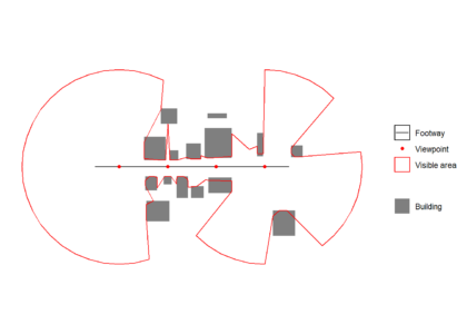
All isovists are unioned to create a visible area polygon, which can see plotted over the original path, viewpoint and building data below.isovists <- do.call(c,isovists)
visareapoly <- st_union(isovists)
ggplot() +
geom_sf(data = buildings,colour = "transparent",aes(fill = 'Building')) +
geom_sf(data = footway, aes(color = 'Footway')) +
geom_sf(data = viewpoints, aes(color = 'Viewpoint')) +
geom_sf(data = visareapoly,fill="transparent",aes(color = 'Visible area')) +
scale_fill_manual(values = c("Building" = "grey50"),
guide = guide_legend(override.aes = list(linetype = c("blank"),
shape = c(NA)))) +
scale_color_manual(values = c("Footway" = "black",
"Viewpoint" = "red",
"Visible area" = "red"),
labels = c("Footway", "Viewpoint","Visible area"))+
guides( color = guide_legend(
order = 1,
override.aes = list(
color = c("black","red","red"),
fill = c("transparent","transparent","white"),
linetype = c("solid","blank", "solid"),
shape = c(NA,16,NA))))+
theme_minimal()+
coord_sf(datum = NA)+
theme(legend.title=element_blank())
Covid-19 shinyapp
The data displayed by this shinyapp is taken from Johns Hopkins University Center for Systems Science and Engineering (JHU CCSE). The raw data is available on
If any further information is needed regarding the data and the application then feel free to send an email to: [email protected]
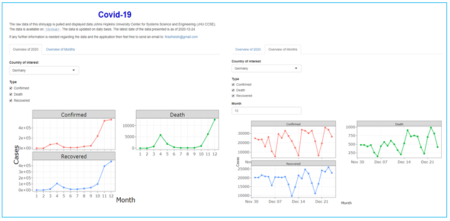
{Github}. The data is updated on daily basis.If any further information is needed regarding the data and the application then feel free to send an email to: [email protected]