If you are building data science applications and need some data to demonstrate the prototype to a potential client, you will most likely need synthetic data. In this article, we discuss the steps to generating synthetic data using the R package ‘conjurer’.
Steps to build synthetic data
1. Installation
Install conjurer package by using the following code. Since the package uses base R functions, it does not have any dependencies.
install.packages("conjurer")
2. Build customers
A customer is identified by a unique customer identifier(ID). A customer ID is alphanumeric with prefix “cust” followed by a numeric. This numeric ranges from 1 and extend to the number of customers provided as the argument within the function. For example, if there are 100 customers, then the customer ID will range from cust001 to cust100. This ensures that the customer ID is always of the same length. Let us build a group of customer IDs using the following code. For simplicity, let us assume that there are 100 customers. customer ID is built using the function
buildCust. This function takes one argument “numOfCust” that specifies the number of customer IDs to be built.
library(conjurer)
customers <- buildCust(numOfCust =  100)
print(head(customers))
#[1] "cust001" "cust002" "cust003" "cust004" "cust005" "cust006"
3. Build products
The next step is building some products. A product is identified by a product ID. Similar to a customer ID, a product ID is also an alphanumeric with prefix “sku” which signifies a stock keeping unit. This prefix is followed by a numeric ranging from 1 and extending to the number of products provided as the argument within the function. For example, if there are 10 products, then the product ID will range from sku01 to sku10. This ensures that the product ID is always of the same length. Besides product ID, the product price range must be specified. Let us build a group of products using the following code. For simplicity, let us assume that there are 10 products and the price range for them is from 5 dollars to 50 dollars. Products are built using the function
buildProd. This function takes 3 arguments as given below.
-
- numOfProd. This defines the number of product IDs to be generated.
- minPrice. This is the minimum value of the price range.
- maxPrice. This is the maximum value of the price range.
library(conjurer)
products <- buildProd(numOfProd = 10, minPrice = 5, maxPrice = 50)
print(head(products))
#     SKU Price
# 1 sku01 43.60
# 2 sku02 48.56
# 3 sku03 36.16
# 4 sku04 19.02
# 5 sku05 17.19
# 6 sku06 25.35
4. Build transactions
Now that a group of customer IDs and Products are built, the next step is to build transactions. Transactions are built using the function genTrans. This function takes 5 arguments. The details of them are as follows.
-
- cylces. This represents the cyclicality of data. It can take the following values
- “y“. If cycles is set to the value “y”, it means that there is only one instance of a high number of transactions during the entire year. This is a very common situation for some retail clients where the highest number of sales are during the holiday period in December.
- “q“. If cycles is set to the value “q”, it means that there are 4 instances of a high number of transactions. This is generally noticed in the financial services industry where the financial statements are revised every quarter and have an impact on the equity transactions in the secondary market.
- “m“. If cycles is set to the value “m”, it means that there are 12 instances of a high number of transactions for a year. This means that the number of transactions increases once every month and then subside for the rest of the month.
- spike. This represents the seasonality of data. It can take any value from 1 to 12. These numbers represent months in an year, from January to December respectively. For example, if spike is set to 12, it means that December has the highest number of transactions.
- trend. This represents the slope of data distribution. It can take a value of 1 or -1.
- If the trend is set to value 1, then the aggregated monthly transactions will exhibit an upward trend from January to December and vice versa if it is set to -1.
- outliers. This signifies the presence of outliers. If set to value 1, then outliers are generated randomly. If set to value 0, then no outliers are generated. The presence of outliers is a very common occurrence and hence setting the outliers to 1 is recommended. However, there are instances where outliers are not needed. For example, if the objective of data generation is solely for visualization purposes then outliers may not be needed.
- transactions. This represents the number of transactions to be generated.
Let us build transactions using the following code
transactions <- genTrans(cycles = "y", spike = 12, outliers = 1, transactions = 10000)
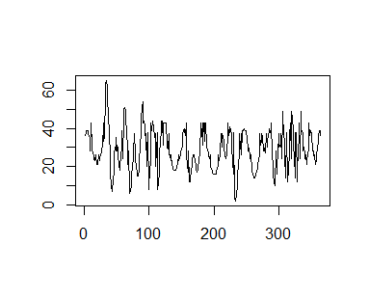
Visualize generated transactions by using
TxnAggregated <- aggregate(transactions$transactionID, by = list(transactions$dayNum), length)
plot(TxnAggregated, type = "l", ann = FALSE)
5. Build final data
Bringing customers, products and transactions together is the final step of generating synthetic data. This process entails 3 steps as given below.
5.1 Allocate customers to transactions
The allocation of transactions is achieved with the help of buildPareto function. This function takes 3 arguments as detailed below.
-
- factor1 and factor2. These are factors to be mapped to each other. As the name suggests, they must be of data type factor.
- Pareto. This defines the percentage allocation and is a numeric data type. This argument takes the form of c(x,y) where x and y are numeric and their sum is 100. If we set Pareto to c(80,20), it then allocates 80 percent of factor1 to 20 percent of factor 2. This is based on a well-known concept of Pareto principle.
Let us now allocate transactions to customers first by using the following code.
customer2transaction <- buildPareto(customers, transactions$transactionID, pareto = c(80,20))
Assign readable names to the output by using the following code.
names(customer2transaction) <- c('transactionID', 'customer')

#inspect the output
print(head(customer2transaction))
#   transactionID customer
# 1     txn-91-11  cust072
# 2    txn-343-25  cust089
# 3    txn-264-08  cust076
# 4    txn-342-07  cust030
# 5      txn-2-19  cust091
# 6    txn-275-06  cust062
5.2 Allocate products to transactions
Now, using similar step as mentioned above, allocate transactions to products using following code.
product2transaction <- buildPareto(products$SKU,transactions$transactionID,pareto = c(70,30))
names(product2transaction) <- c('transactionID', 'SKU')

#inspect the output
print(head(product2transaction))
#   transactionID   SKU
# 1    txn-182-30 sku10
# 2    txn-179-21 sku01
# 3    txn-179-10 sku10
# 4    txn-360-08 sku01
# 5     txn-23-09 sku01
# 6    txn-264-20 sku10
5.3 Final data
Now, using a similar step as mentioned above, allocate transactions to products using the following code.
df1 <- merge(x = customer2transaction, y = product2transaction, by = "transactionID")

dfFinal <- merge(x = df1, y = transactions, by = "transactionID", all.x = TRUE)

#inspect the output
print(head(dfFinal))
#   transactionID customer   SKU dayNum mthNum
# 1      txn-1-01  cust076 sku03      1      1
# 2      txn-1-02  cust062 sku04      1      1
# 3      txn-1-03  cust087 sku07      1      1
# 4      txn-1-04  cust010 sku04      1      1
# 5      txn-1-05  cust039 sku01      1      1
# 6      txn-1-06  cust010 sku01      1      1
Thus, we have the final data set with transactions, customers and products. Interpret the results The column names of the final data frame can be interpreted as follows.
-
- Each row is a transaction and the data frame has all the transactions for a year i.e 365 days.
- transactionID is the unique identifier for that transaction. + customer is the unique customer identifier. This is the customer who made that transaction.
- SKU is the product that was bought in that transaction.
- dayNum is the day number in the year. There would be 365 unique dayNum in the data frame.
- mthNum is the month number. This ranges from 1 to 12 and represents January to December respectively.
Summary & concluding remarks
In this article, we started by building customers, products and transactions. Later on, we also understood how to bring them all together in to a final data set. At the time of writing this article, the package is predominantly focused on building the basic data set and there is room for improvement. If you are interested in contributing to this package, please find the details at
contributions.