Find the next number in the sequence

Find the next number in the sequence
by Jerry Tuttle

Between ages two and four, most children can count up to at 
least ten.  If you ask your child, "What number comes next after 1, 2, 3, 4, 5?" they will probably say "6."

But to math nerds, any number can be the next number in a finite sequence. I like -14.

Given a sequence of n real numbers f(x1), f(x2), f(x3), ... , f(xn), there is always a mathematical procedure to find the next number f(x n+1) of the sequence. The resulting solution may not appear to be satisfying to students, but it is mathematically logical.

I can draw a smooth curve through the points (1,1), (2,2), (3,3), (4,4), (5,5), (6, -14). If I can find an equation for that smooth curve, then I know my answer of -14 has some logic to it. Actually many equations will work.

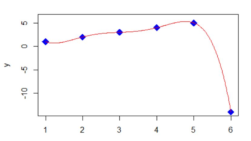
In my example one equation is of the form y = (x-1)*(x-2)*(x-3)*(x-4)*(x-5)*(A/120) + x, where A is chosen so that when x is 6, the first term reduces to A, and A + 6 equals the -14 I want. So A is -20. This is called a collocation polynomial.

There is a theorem that for n+1 distinct values of xi and their corresponding yi values, there is a unique polynomial P of degree n with P(xi) = yi. One method to find P is to use polynomial regression. Another way is to use Newton's Forward Difference Formula (probably no longer taught in Numerical Analysis courses).

Higher degree polynomials than degree n is one reason why additional equations will work.

The equation does not have to be a polynomial, which then adds rational functions among others.

Of course the next number after -14 can be any number. It could be 7 :)

There are many famous sequences, and of course someone catalogued  them.

Here is some R code.

xpoints <- c(1,2,3,4,5,6)
ypoints <- c(1,2,3,4,5,-14)
y <- vector()
x <- seq(from=1, to=6, by=.01)
y <- (x-1)*(x-2)*(x-3)*(x-4)*(x-5)*(-20/120) + x
plot(xpoints, ypoints, pch=18, type="p", cex=2, col="blue", xlim=c(1,6), ylim=c(-14,6), xlab="x", ylab="y")
lines(x,y, pch = 19, cex=1.3, col = "red")
fit <- lm(ypoints ~ xpoints + I(xpoints^2) + I(xpoints^3) +I(xpoints^4) +I(xpoints^5) )
s <- summary(fit)
bo <- s$coefficient[1]
b1 <- s$coefficient[2]
b2 <- s$coefficient[3]
b3 <- s$coefficient[4]
b4 <- s$coefficient[5]
b5 <- s$coefficient[6]
x <- seq(from=1, to=6, by=.01)
z <- bo+b1*x+b2*x^2+b3*x^3+b4*x^4+b5*x^5
plot(xpoints, ypoints, pch=18, type="p", cex=2, col="blue", xlim=c(1,6), ylim=c(-14,6), xlab="x", ylab="y")
lines(x,z, pch = 19, cex=1.3, col = "red")