Computation time of loops — for, *apply, map

It is usually said, that for– and while-loops should be avoided in R. I was curious about just how the different alternatives compare in terms of speed.

The first loop is perhaps the worst I can think of – the return vector is initialized without type and length so that the memory is constantly being allocated.
use_for_loop <- function(x){
  y <- c()
  
  for(i in x){
    y <- c(y, x[i] * 100)
  }
  return(y)
}
The second for loop is with preallocated size of the return vector.
use_for_loop_vector <- function(x){
  y <- vector(mode = "double", length = length(x))
  
  for(i in x){
    y[i] <- x[i] * 100
  }
  return(y)
}
I have noticed I use sapply() quite a lot, but I think not once have I used vapply() We will nonetheless look at both
use_sapply <- function(x){
  sapply(x, function(y){y * 100})
}


use_vapply <- function(x){
  vapply(x, function(y){y * 100}, double(1L))
}
And because I am a tidyverse-fanboy we also loop at map_dbl().
library(purrr)
use_map_dbl <- function(x){
  map_dbl(x, function(y){y * 100})
}
We test the functions using a vector of random doubles and evaluate the runtime with microbenchmark.
x <- c(rnorm(100))
mb_res <- microbenchmark::microbenchmark(
  `for_loop()` = use_for_loop(x),
  `for_loop_vector()` = use_for_loop_vector(x),
  `purrr::map_dbl()` = use_map_dbl(x),
  `sapply()` = use_sapply(x),
  `vapply()` = use_vapply(x),
  times = 500
)
The results are listed in table and figure below.
expr min lq mean median uq max neval
for_loop() 8.440 9.7305 10.736446 10.2995 10.9840 26.976 500
for_loop_vector() 10.912 12.1355 13.468312 12.7620 13.8455 37.432 500
purrr::map_dbl() 22.558 24.3740 25.537080 25.0995 25.6850 71.550 500
sapply() 15.966 17.3490 18.483216 18.1820 18.8070 59.289 500
vapply() 6.793 8.1455 8.592576 8.5325 8.8300 26.653 500

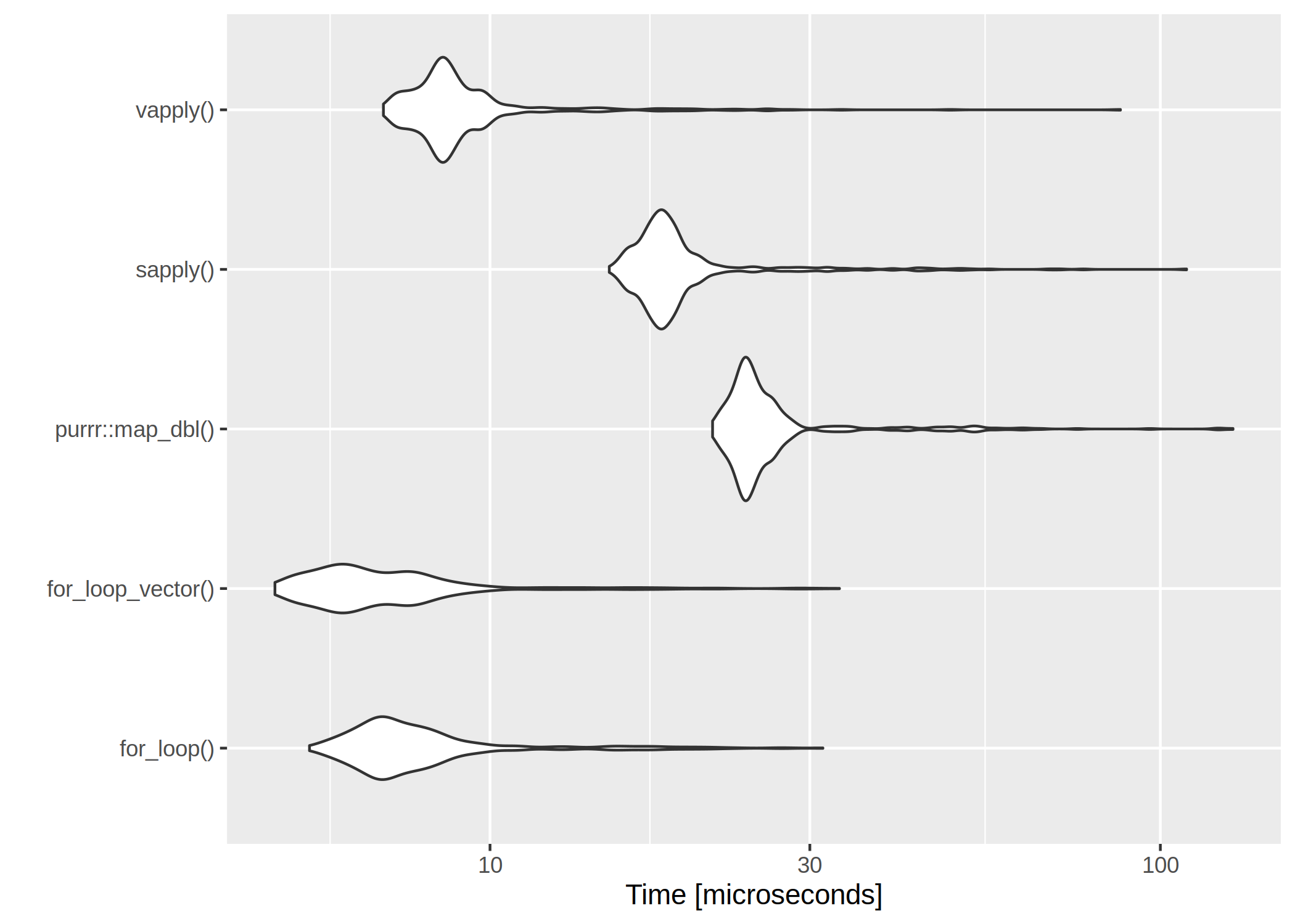
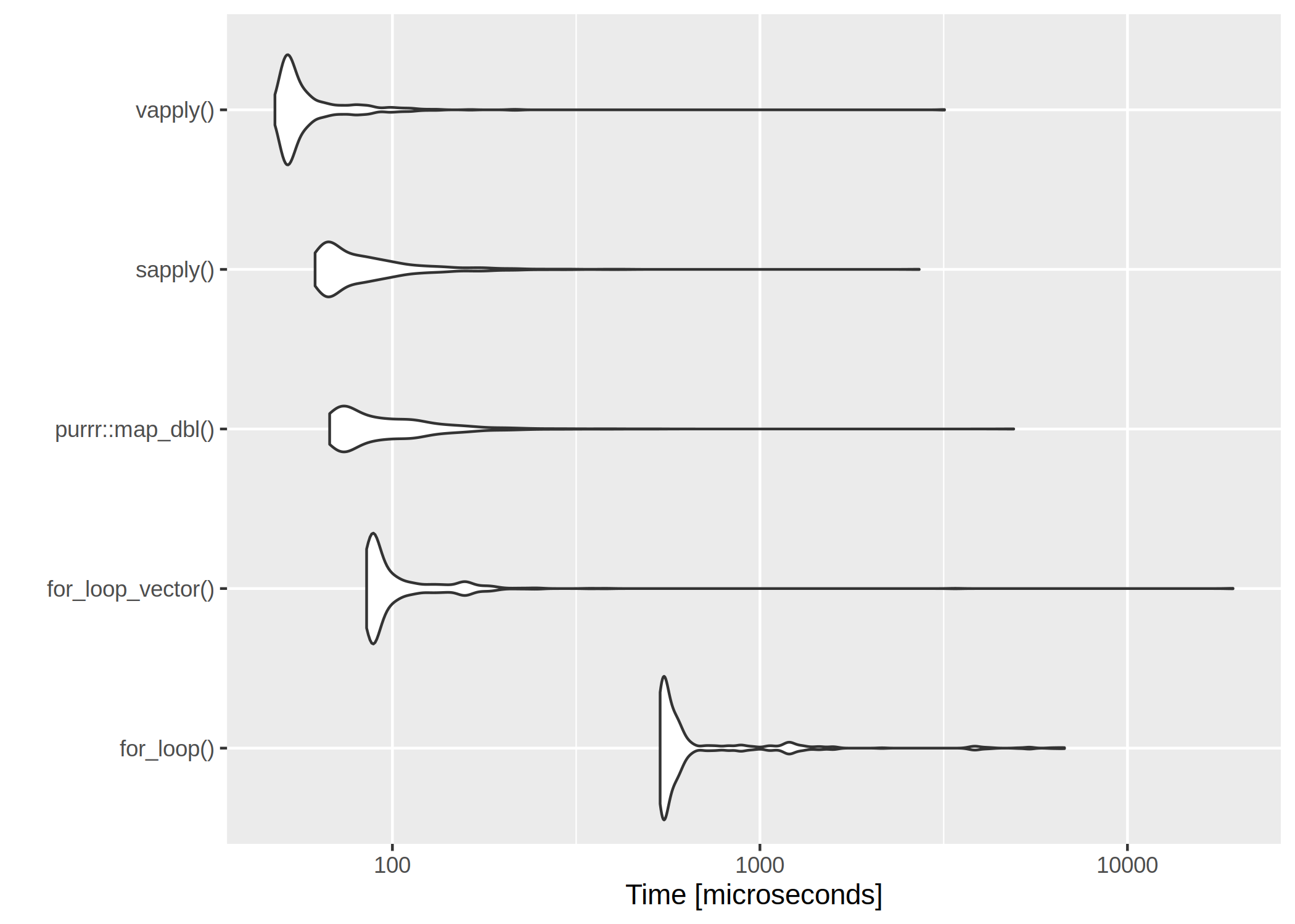
  The clear winner is vapply() and for-loops are rather slow. However, if we have a very low number of iterations, even the worst for-loop isn’t too bad:
x <- c(rnorm(10))
mb_res <- microbenchmark::microbenchmark(
  `for_loop()` = use_for_loop(x),
  `for_loop_vector()` = use_for_loop_vector(x),
  `purrr::map_dbl()` = use_map_dbl(x),
  `sapply()` = use_sapply(x),
  `vapply()` = use_vapply(x),
  times = 500
)
expr min lq mean median uq max neval
for_loop() 5.992 7.1185 9.670106 7.9015 9.3275 70.955 500
for_loop_vector() 5.743 7.0160 9.398098 7.9575 9.2470 40.899 500
purrr::map_dbl() 22.020 24.1540 30.565362 25.1865 27.5780 157.452 500
sapply() 15.456 17.4010 22.507534 18.3820 20.6400 203.635 500
vapply() 6.966 8.1610 10.127994 8.6125 9.7745 66.973 500

Benchmarking cast in R from long data frame to wide matrix

In my daily work I often have to transform a long table to a wide matrix so accommodate some function. At some stage in my life I came across the reshape2 package, and I have been with that philosophy ever since – I find it makes data wrangling easy and straight forward. I particularly like the tidyverse philosophy where data should be in a long table, where one row is an observation, and a column a parameter. It just makes sense.

However, I quite often have to transform the data into another format, a wide matrix especially for functions of the vegan package, and one day I wondering how to do that in the fastest way.

The code to create the test sets and benchmark the functions is in section ‘Settings and script’ at the end of this document.

I created several data sets that mimic the data I usually work with in terms of size and values. The data sets have 2 to 10 groups, where each group can have up to 50000, 100000, 150000, or 200000 samples. The methods xtabs() from base R, dcast() from data.table, dMcast() from Matrix.utils, and spread() from tidyr were benchmarked using microbenchmark() from the package microbenchmark. Each method was evaluated 10 times on the same data set, which was repeated for 10 randomly generated data sets.

After the 10 x 10 repetitions of casting from long to wide it is clear the spread() is the worst. This is clear when we focus on the size (figure 1).
Figure 1. Runtime for 100 repetitions of data sets of different size and complexity.
And the complexity (figure 2).
Figure 2. Runtime for 100 repetitions of data sets of different complexity and size.

Close up on the top three methods

Casting from a long table to a wide matrix is clearly slowest with spread(), where as the remaining look somewhat similar. A direct comparison of the methods show a similarity in their performance, with dMcast() from the package Matrix.utils being better — especially with the large and more complex tables (figure 3).
Figure 3. Direct comparison of set size.
I am aware, that it might be to much to assume linearity, between the computation times at different set sizes, but I do believe it captures the point – dMcast() and dcast() are similar, with advantage to dMcast() for large data sets with large number of groups. It does, however, look like dcast() scales better with the complexity (figure 4).
Figure 4. Direct comparison of number groups.

Settings and script

Session info

 ## ─ Session info ──────────────────────────────────────────────────────────
 ## setting value 
 ## version R version 3.5.2 (2018-12-20)
 ## os Ubuntu 18.04.1 LTS 
 ## system x86_64, linux-gnu 
 ## ui X11 
 ## language en_GB:en_US 
 ## collate en_DE.UTF-8 
 ## ctype en_DE.UTF-8 
 ## tz Europe/Berlin 
 ## date 2019-02-03 
 ## 
 ## ─ Packages ──────────────────────────────────────────────────────────────
 ## package * version date lib source 
 ## assertthat 0.2.0 2017-04-11 [1] CRAN (R 3.5.2)
 ## bindr 0.1.1 2018-03-13 [1] CRAN (R 3.5.2)
 ## bindrcpp * 0.2.2 2018-03-29 [1] CRAN (R 3.5.2)
 ## cli 1.0.1 2018-09-25 [1] CRAN (R 3.5.2)
 ## colorspace 1.4-0 2019-01-13 [1] CRAN (R 3.5.2)
 ## crayon 1.3.4 2017-09-16 [1] CRAN (R 3.5.2)
 ## digest 0.6.18 2018-10-10 [1] CRAN (R 3.5.2)
 ## dplyr * 0.7.8 2018-11-10 [1] CRAN (R 3.5.2)
 ## evaluate 0.12 2018-10-09 [1] CRAN (R 3.5.2)
 ## ggplot2 * 3.1.0 2018-10-25 [1] CRAN (R 3.5.2)
 ## glue 1.3.0 2018-07-17 [1] CRAN (R 3.5.2)
 ## gtable 0.2.0 2016-02-26 [1] CRAN (R 3.5.2)
 ## highr 0.7 2018-06-09 [1] CRAN (R 3.5.2)
 ## htmltools 0.3.6 2017-04-28 [1] CRAN (R 3.5.2)
 ## knitr 1.21 2018-12-10 [1] CRAN (R 3.5.2)
 ## labeling 0.3 2014-08-23 [1] CRAN (R 3.5.2)
 ## lazyeval 0.2.1 2017-10-29 [1] CRAN (R 3.5.2)
 ## magrittr 1.5 2014-11-22 [1] CRAN (R 3.5.2)
 ## munsell 0.5.0 2018-06-12 [1] CRAN (R 3.5.2)
 ## packrat 0.5.0 2018-11-14 [1] CRAN (R 3.5.2)
 ## pillar 1.3.1 2018-12-15 [1] CRAN (R 3.5.2)
 ## pkgconfig 2.0.2 2018-08-16 [1] CRAN (R 3.5.2)
 ## plyr 1.8.4 2016-06-08 [1] CRAN (R 3.5.2)
 ## purrr 0.2.5 2018-05-29 [1] CRAN (R 3.5.2)
 ## R6 2.3.0 2018-10-04 [1] CRAN (R 3.5.2)
 ## Rcpp 1.0.0 2018-11-07 [1] CRAN (R 3.5.2)
 ## rlang 0.3.1 2019-01-08 [1] CRAN (R 3.5.2)
 ## rmarkdown 1.11 2018-12-08 [1] CRAN (R 3.5.2)
 ## scales 1.0.0 2018-08-09 [1] CRAN (R 3.5.2)
 ## sessioninfo 1.1.1 2018-11-05 [1] CRAN (R 3.5.2)
 ## stringi 1.2.4 2018-07-20 [1] CRAN (R 3.5.2)
 ## stringr * 1.3.1 2018-05-10 [1] CRAN (R 3.5.2)
 ## tibble 2.0.1 2019-01-12 [1] CRAN (R 3.5.2)
 ## tidyselect 0.2.5 2018-10-11 [1] CRAN (R 3.5.2)
 ## viridisLite 0.3.0 2018-02-01 [1] CRAN (R 3.5.2)
 ## withr 2.1.2 2018-03-15 [1] CRAN (R 3.5.2)
 ## xfun 0.4 2018-10-23 [1] CRAN (R 3.5.2)
 ## yaml 2.2.0 2018-07-25 [1] CRAN (R 3.5.2)

Settings

# settings.yml
set_size: [50000, 100000, 150000, 200000]
num_groups: [2, 3, 4, 5, 6, 7, 8, 9, 10]
benchmark_repetitions: 10
num_test_sets: 10
max_value: 500
word_length: 10

Data creation and benchmarking scripts

# main.R
# Global variables ----------------------------------------------
# Set this to FALSE if you want to run the complete analysis
running_test <- TRUE
vars <- yaml::read_yaml("./settings.yml")
set_size <- vars$set_size
num_groups <- vars$num_groups
benchmark_repetitions <- vars$benchmark_repetitions
num_test_sets <- vars$num_test_sets
max_value <- vars$max_value
word_length <- vars$word_length

# Test variables ------------------------------------------------
if(running_test){
set_size <- seq.int(0L, 60L, 30L)
num_groups <- c(2L:3L)
benchmark_repetitions <- 2L
num_test_sets <- 2L
}


# Libraries ----------------------------------------------------- 
suppressPackageStartupMessages(library(foreach))
suppressPackageStartupMessages(library(doParallel))


# Setup parallel ------------------------------------------------
num_cores <- detectCores() - 1

these_cores <- makeCluster(num_cores, type = "PSOCK")
registerDoParallel(these_cores)

# Functions -----------------------------------------------------
run_benchmark <- function(as){
source("test_cast.R")
num_groups <- as["num_groups"]
set_size <- as["set_size"]
num_test_sets <- as["num_test_sets"]
word_length <- as["word_length"]
max_value <- as["max_value"]
 
test_data <- prepare_test_data(set_size, num_groups, word_length, max_value)
perform_benchmark(test_data, benchmark_repetitions)
}


# Setup and run tests -------------------------------------------
set_size <- set_size[set_size > 0]

analysis_comb <- expand.grid(num_groups, set_size)
analysis_settings <- vector("list", length = nrow(analysis_comb))

for(i in seq_len(nrow(analysis_comb))){
analysis_settings[[i]] <- c(num_groups =analysis_comb[i, "Var1"],
set_size = analysis_comb[i, "Var2"],
word_length = word_length,
max_value = max_value,
benchmark_repetitions = benchmark_repetitions)
}


for(as in analysis_settings){
num_groups <- as["num_groups"]
set_size <- as["set_size"]

report_str <- paste("ng:", num_groups,
"- setsize:", set_size, "\n")
cat(report_str)
 
rds_file_name <- paste0("./output/benchmark_setsize-", set_size,
"_ng-", num_groups, ".rds")
 
bm_res <- foreach(seq_len(num_test_sets), .combine = "rbind") %dopar% {
run_benchmark(as)
 }
 
bm_res <- dplyr::mutate(bm_res, `Number groups` = num_groups,
 `Set size` = set_size)
 
saveRDS(bm_res, rds_file_name)
report_str
}
# test_cast.R
setup <- function(){
library(data.table)
library(tidyr)
library(dplyr)
library(Matrix.utils)
library(tibble)
}

prepare_test_data <- function(set_size, num_groups, word_length, sample_int_n){
calc_subset_size <- function(){
subset_size <- 0
while(subset_size == 0 | subset_size > set_size){
subset_size <- abs(round(set_size - set_size/(3 + rnorm(1))))
 }
subset_size
 }
 
words <- stringi::stri_rand_strings(set_size, word_length)
subset_sizes <- replicate(num_groups, calc_subset_size())
 
 purrr::map_df(subset_sizes, function(subset_size){
 tibble::tibble(Variable = sample(words, subset_size),
Value = sample.int(sample_int_n, subset_size, replace = TRUE),
Group = stringi::stri_rand_strings(1, word_length))
 })
}

test_tidyr <- function(test_df){
test_df %>% 
spread(Variable, Value, fill = 0L) %>% 
 tibble::column_to_rownames(var = "Group") %>% 
as.matrix.data.frame()
}

test_xtabs <- function(test_df){
xtabs(Value ~ Group + Variable, data = test_df) 
}

test_dMcast <- function(test_df){
class(test_df) <- "data.frame"
dMcast(test_df, Group ~ Variable, value.var = "Value")
}

test_dcast <- function(test_df){
test_df_dt <- data.table(test_df)
dcast(test_df_dt, Group ~ Variable, value.var = "Value", fill = 0) %>% 
 tibble::column_to_rownames(var = "Group") %>% 
as.matrix.data.frame()
}


perform_benchmark <- function(test_df, benchmark_repetitions){
suppressPackageStartupMessages(setup())
bm_res <- microbenchmark::microbenchmark(
Spread = test_tidyr(test_df = test_df), 
Xtabs = test_xtabs(test_df = test_df), 
dMcast = test_dMcast(test_df = test_df), 
dcast = test_dcast(test_df = test_df), 
times = benchmark_repetitions
 )
class(bm_res) <- "data.frame"
 
bm_res %>% 
mutate(time = microbenchmark:::convert_to_unit(time, "ms")) %>% 
rename(Method = expr, `Time (ms)` = time)
}

GitLab CI for R-package development

— A basic R-phile introduction to continuous integration on GitLab

I have been using the GitLab repository for some time for mainly two reasons: I can have private projects at no monetary costs (I later came to realise that I as an academic can have the same on GitHub), and most importantly GitLab has so far gone under the radar of our IT department, meaning I can access it from my work computer. GitHub on the other hand is flagged as file sharing.

A simple CI config

Most of my time with R is spend trying to make heads and tails of various kinds of data, and I have so far just authored one R-package. While I can see the benefits of a continuous integration (CI) work flow, I just never bothered to actually set it up. Now where I am putting together code in smaller packages for internal use, it seemed like the right time to learn a little.

The Internet gives a few pointers on how to go about setting up CI on GitLab; one of the resources is the blog post Docker, GitLab CI and Developing R Packages by Mustafa Hasanbulli, who gives a simple .gitlab-ci.yml for testing packages. Mustafa’s solution make use of the rocker/tidyverse Docker image and install the dependency packages before running check() from devtools. It’s a good solution and combining with the .gitlab-ci.yml shared as a gist on Github by Artem Klevtsov, I managed to get the coverage badge I though nice to have. The .gitlab-ci.yml for a smaller package can be along the lines of:

image: rocker/tidyverse

stages:
  - check
  - coverage

check_pkg:
  stage: check
  script:
    - R -e 'install.packages(c())'
    - R -e 'devtools::check()'

coverage:
   stage: coverage
   script:
     - R -e 'covr::package_coverage(type = c("tests", "examples"))'

To extract the coverage to the coverage badge, add Coverage: \d+.\d+%$ to the section ‘Test coverage parsing’ in Settings -> CI/CD -> General pipelines.

Introducing cache

For my package, each of the two stages took about 45 minutes to complete, and I realized that the wast majority of the time was spent on downloading and especially installing packages. This was mainly do to the Bioconductor packages I rely on.

If only there would be a way to pass the installed packages between the stages, or even between runs of the CI pipeline. There is – GitLab 9.0 saw the option to specify a cache. The next problem is that the cache must be a directory of the cloned project directory. Since R prefers to install packages in /usr/lib/R/library in the Docker images, the .libpaths() must be changed. In addition you would have to remember to add any new package to the .gitlab-ci.yml. Which I for one would always forget, and therefore painstakingly have to figure out which packages to add.

A much simpler solution is to use packrat – something you anyway should consider to use. It also allows you to use the rocker/r-base image and just the packages actually required for your CI. How much of a win in terms of traffic rocker/r-base is over rocker/tidyverse probably depends on the packages you have to add. The .gitlab-ci.yml caching packages could look like this:

image: rocker/r-base

stages:
  - setup
  - test

cache:
  # Ommit key to use the same cache across all pipelines and branches
  key: "$CI_COMMIT_REF_SLUG"
  paths:
    - packrat/lib/

setup:
  stage: setup
  script:
    - R -e 'source("ci.R"); ci_setup()'

check:
  stage: test
  dependencies:
    - setup
  when: on_success
  script:
    - R -e 'source("ci.R"); ci_check()'

coverage:
  stage: test
  dependencies:
    - setup
  when: on_success
  only:
    - master
  script:
    - R -e 'source("ci.R"); ci_coverage()'

with the ci.R looking like this:

install_if_needed <- function(package_to_install){
  package_path <- find.package(package_to_install, quiet = TRUE)

  if(length(package_path) == 0){
    # Only install if not present
    install.packages(package_to_install)
  }
}

ci_setup <- function(){
  install_if_needed("packrat")
  packrat::restore()
}

ci_check <- function(){
  install_if_needed("devtools")
  devtools::check()
}

ci_coverage <- function(){
  install_if_needed("covr")
  covr::package_coverage(type = c("tests", "examples"))
}

The cache key $CI_COMMIT_REF_SLUG gives you the advantage of different cache for different branches. Using $CI_COMMIT_SHA will give you a separate cache for each commit.

Adding the packrat subdirectories src and lib* to the .gitignore will keep your repository small – and I find it quite useful to commit just the packrat.lock whenever I add or remove a package. But then again, I am the only one working with my repositories, and there might be advantages I don’t know of.

I have noticed that the stages after the setup stage sometimes fail in the first run. If this happens because of the cache, rerunning the failed stage makes everything well.

Using the above for my package, the first run of the pipeline took about 45 minutes, but the second run only about 8 minutes. A considerable reduction in time.

I hope .gitlab-ci.yml and ci.R outlined here will help you getting started on caching your R-packages in your CI. The two modules are quite simple, and if you are loking for something more sophisticated, I can recommend looking Matt Dowle works on data.table and of course the GitLab Runner help pages.