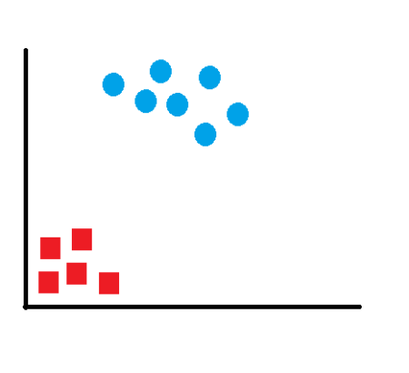
Have you ever wondered why do we ask multiple people about their opinions or reviews before going for a movie or before buying a car or may be, before planning a holiday? It’s because review of one person may be biased as per her preference; however, when we ask multiple people we are trying to remove bias that a single person may provide. One person may have a very strong dislike for a specific destination because of her experience at that location; however, ten other people may have very strong preference for the same destination because they have had a wonderful experience there. From this, we can infer that the one person was more like an exceptional case and her experience may be one of a case.
Another example which I am sure all of us have encountered is during the interviews at any company or college. We often have to go through multiple rounds of interviews. Even though the questions asked in multiple rounds of interview are similar, if not same – companies still go for it. The reason is that they want to have views from multiple recruitment leaders. If multiple leaders are zeroing in on a candidate then the likelihood of her turning out to be a good hire is high.
In the world of analytics and data science, this is called ‘ensembling’. Ensembling is a “type of supervised learning technique where multiple models are trained on a training dataset and their individual outputs are combined by some rule to derive the final output.”
Let’s break the above definition and look at it step by step.
When we say multiple models are trained on a dataset, same model with different hyper parameters or different models can be trained on the training dataset. Training observations may differ slightly while sampling; however, overall population remains the same.
“Outputs are combined by some rule” – there could be multiple rules by which outputs are combined. The most common ones are the average (in terms of numerical output) or vote (in terms of categorical output). When different models give us numerical output, we can simply take the average of all the outputs and use the average as the result. In case of categorical output, we can use vote – output occurring maximum number of times is the final output. There are other complex methods of deriving at output also but they are out of scope of this article.
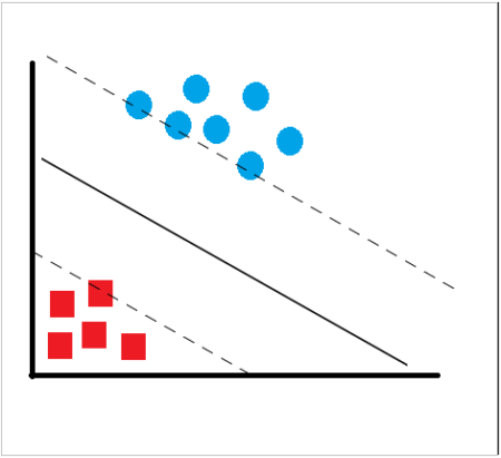
Random Forest is one such very powerful ensembling machine learning algorithm which works by creating multiple decision trees and then combining the output generated by each of the decision trees. Decision tree is a classification model which works on the concept of information gain at every node. For all the data points, decision tree will try to classify data points at each of the nodes and check for information gain at each node. It will then classify at the node where information gain is maximum. It will follow this process subsequently until all the nodes are exhausted or there is no further information gain. Decision trees are very simple and easy to understand models; however, they have very low predictive power. In fact, they are called weak learners.
Random Forest works on the same weak learners. It combines the output of multiple decision trees and then finally come up with its own output. Random Forest works on the same principle as Decision Tress; however, it does not select all the data points and variables in each of the trees. It randomly samples data points and variables in each of the tree that it creates and then combines the output at the end. It removes the bias that a decision tree model might introduce in the system. Also, it improves the predictive power significantly. We will see this in the next section when we take a sample data set and compare the accuracy of Random Forest and Decision Tree.
Now, let’s take a small case study and try to implement multiple Random Forest models with different hyper parameters, and compare one of the Random Forest model with Decision Tree model. (I am sure you will agree with me on this – even without implementing the model, we can say intuitively that Random Forest will give us better results than Decision Tree). The dataset is taken from UCI website and can be found on this link. The data contains 7 variables – six explanatory (Buying Price, Maintenance, NumDoors, NumPersons, BootSpace, Safety) and one response variable (Condition). The variables are self-explanatory and refer to the attributes of cars and the response variable is ‘Car Acceptability’. All the variables are categorical in nature and have 3-4 factor levels in each.
Let’s start the R code implementation and predict the car acceptability based on explanatory variables.
# Data Source: https://archive.ics.uci.edu/ml/machine-learning-databases/car/

install.packages("randomForest")
library(randomForest)
# Load the dataset and explore
data1 <- read.csv(file.choose(), header = TRUE)

head(data1)

str(data1)

summary(data1)
> head(data1)
  BuyingPrice Maintenance NumDoors NumPersons BootSpace Safety Condition
1       vhigh       vhigh        2          2     small    low     unacc
2       vhigh       vhigh        2          2     small    med     unacc
3       vhigh       vhigh        2          2     small   high     unacc
4       vhigh       vhigh        2          2       med    low     unacc
5       vhigh       vhigh        2          2       med    med     unacc
6       vhigh       vhigh        2          2       med   high     unacc
> str(data1)
'data.frame':   1728 obs. of  7 variables:
 $ BuyingPrice: Factor w/ 4 levels "high","low","med",..: 4 4 4 4 4 4 4 4 4 4 ...
 $ Maintenance: Factor w/ 4 levels "high","low","med",..: 4 4 4 4 4 4 4 4 4 4 ...
 $ NumDoors   : Factor w/ 4 levels "2","3","4","5more": 1 1 1 1 1 1 1 1 1 1 ...
 $ NumPersons : Factor w/ 3 levels "2","4","more": 1 1 1 1 1 1 1 1 1 2 ...
 $ BootSpace  : Factor w/ 3 levels "big","med","small": 3 3 3 2 2 2 1 1 1 3 ...
 $ Safety     : Factor w/ 3 levels "high","low","med": 2 3 1 2 3 1 2 3 1 2 ...
 $ Condition  : Factor w/ 4 levels "acc","good","unacc",..: 3 3 3 3 3 3 3 3 3 3 ...
> summary(data1)
 BuyingPrice Maintenance  NumDoors   NumPersons BootSpace    Safety    Condition
 high :432   high :432   2    :432   2   :576   big  :576   high:576   acc  : 384
 low  :432   low  :432   3    :432   4   :576   med  :576   low :576   good :  69
 med  :432   med  :432   4    :432   more:576   small:576   med :576   unacc:1210
 vhigh:432   vhigh:432   5more:432                                     vgood:  65
Now, we will split the dataset into train and validation set in the ratio 70:30. We can also create a test dataset, but for the time being we will just keep train and validation set.
# Split into Train and Validation sets
# Training Set : Validation Set = 70 : 30 (random)
set.seed(100)
train <- sample(nrow(data1), 0.7*nrow(data1), replace = FALSE)
TrainSet <- data1[train,]
ValidSet <- data1[-train,]
summary(TrainSet)
summary(ValidSet)
> summary(TrainSet)
 BuyingPrice Maintenance  NumDoors   NumPersons BootSpace    Safety    Condition
 high :313   high :287   2    :305   2   :406   big  :416   high:396   acc  :264
 low  :292   low  :317   3    :300   4   :399   med  :383   low :412   good : 52
 med  :305   med  :303   4    :295   more:404   small:410   med :401   unacc:856
 vhigh:299   vhigh:302   5more:309                                     vgood: 37
> summary(ValidSet)
 BuyingPrice Maintenance  NumDoors   NumPersons BootSpace    Safety    Condition
 high :119   high :145   2    :127   2   :170   big  :160   high:180   acc  :120
 low  :140   low  :115   3    :132   4   :177   med  :193   low :164   good : 17
 med  :127   med  :129   4    :137   more:172   small:166   med :175   unacc:354
 vhigh:133   vhigh:130   5more:123                                     vgood: 28
Now, we will create a Random Forest model with default parameters and then we will fine tune the model by changing ‘mtry’. We can tune the random forest model by changing the number of trees (ntree) and the number of variables randomly sampled at each stage (mtry). According to Random Forest package description:
Ntree: Number of trees to grow. This should not be set to too small a number, to ensure that every input row gets predicted at least a few times.
Mtry: Number of variables randomly sampled as candidates at each split. Note that the default values are different for classification (sqrt(p) where p is number of variables in x) and regression (p/3)
# Create a Random Forest model with default parameters
model1 <- randomForest(Condition ~ ., data = TrainSet, importance = TRUE)
model1
> model1

Call:
 randomForest(formula = Condition ~ ., data = TrainSet, importance = TRUE)
               Type of random forest: classification
                     Number of trees: 500
No. of variables tried at each split: 2

        OOB estimate of  error rate: 3.64%
Confusion matrix:
      acc good unacc vgood class.error
acc   253    7     4     0  0.04166667
good    3   44     1     4  0.15384615
unacc  18    1   837     0  0.02219626
vgood   6    0     0    31  0.16216216
By default, number of trees is 500 and number of variables tried at each split is 2 in this case. Error rate is 3.6%.
# Fine tuning parameters of Random Forest model
model2 <- randomForest(Condition ~ ., data = TrainSet, ntree = 500, mtry = 6, importance = TRUE)
model2
> model2

Call:
 randomForest(formula = Condition ~ ., data = TrainSet, ntree = 500,      mtry = 6, importance = TRUE)
               Type of random forest: classification
                     Number of trees: 500
No. of variables tried at each split: 6

        OOB estimate of  error rate: 2.32%
Confusion matrix:
      acc good unacc vgood class.error
acc   254    4     6     0  0.03787879
good    3   47     1     1  0.09615385
unacc  10    1   845     0  0.01285047
vgood   1    1     0    35  0.05405405
When we have increased the mtry to 6 from 2, error rate has reduced from 3.6% to 2.32%. We will now predict on the train dataset first and then predict on validation dataset.
# Predicting on train set
predTrain <- predict(model2, TrainSet, type = "class")
# Checking classification accuracy
table(predTrain, TrainSet$Condition)
> table(predTrain, TrainSet$Condition)

predTrain acc good unacc vgood
    acc   264    0     0     0
    good    0   52     0     0
    unacc   0    0   856     0
    vgood   0    0     0    37
# Predicting on Validation set
predValid <- predict(model2, ValidSet, type = "class")
# Checking classification accuracy
mean(predValid == ValidSet$Condition)
table(predValid,ValidSet$Condition)
> mean(predValid == ValidSet$Condition)
[1] 0.9884393
> table(predValid,ValidSet$Condition)

predValid acc good unacc vgood
    acc   117    0     2     0
    good    1   16     0     0
    unacc   1    0   352     0
    vgood   1    1     0    28
In case of prediction on train dataset, there is zero misclassification; however, in the case of validation dataset, 6 data points are misclassified and accuracy is 98.84%. We can also use function to check important variables. The below functions show the drop in mean accuracy for each of the variables.
# To check important variables
importance(model2)
varImpPlot(model2)
> importance(model2)
                  acc     good     unacc    vgood MeanDecreaseAccuracy MeanDecreaseGini
BuyingPrice 143.90534 80.38431 101.06518 66.75835            188.10368         71.15110
Maintenance 130.61956 77.28036  98.23423 43.18839            171.86195         90.08217
NumDoors     32.20910 16.14126  34.46697 19.06670             49.35935         32.45190
NumPersons  142.90425 51.76713 178.96850 49.06676            214.55381        125.13812
BootSpace    85.36372 60.34130  74.32042 50.24880            132.20780         72.22591
Safety      179.91767 93.56347 207.03434 90.73874            275.92450        149.74474
> varImpPlot(model2)Now, we will use ‘for’ loop and check for different values of mtry.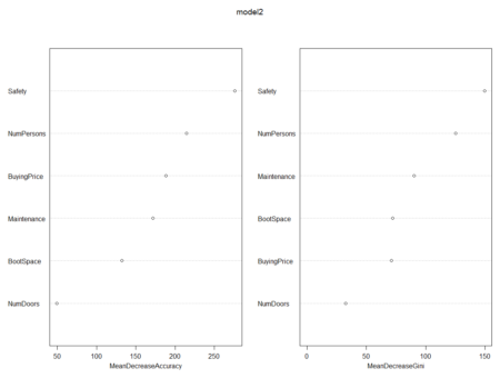
# Using For loop to identify the right mtry for model
a=c()
i=5
for (i in 3:8) {
  model3 <- randomForest(Condition ~ ., data = TrainSet, ntree = 500, mtry = i, importance = TRUE)
  predValid <- predict(model3, ValidSet, type = "class")
  a[i-2] = mean(predValid == ValidSet$Condition)
}

a

plot(3:8,a)
> a
[1] 0.9749518 0.9884393 0.9845857 0.9884393 0.9884393 0.9903661
>
> plot(3:8,a)
From the above graph, we can see that the accuracy decreased when mtry was increased from 4 to 5 and then increased when mtry was changed to 6 from 5. Maximum accuracy is at mtry equal to 8.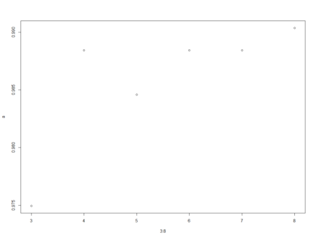
Now, we have seen the implementation of Random Forest and understood the importance of the model. Let’s compare this model with decision tree and see how decision trees fare in comparison to random forest.
# Compare with Decision Tree

install.packages("rpart")
install.packages("caret")
install.packages("e1071")

library(rpart)
library(caret)
library(e1071)
# We will compare model 1 of Random Forest with Decision Tree model

model_dt = train(Condition ~ ., data = TrainSet, method = "rpart")
model_dt_1 = predict(model_dt, data = TrainSet)
table(model_dt_1, TrainSet$Condition)

mean(model_dt_1 == TrainSet$Condition)
> table(model_dt_1, TrainSet$Condition)

model_dt_1 acc good unacc vgood
     acc   241   52   132    37
     good    0    0     0     0
     unacc  23    0   724     0
     vgood   0    0     0     0
>
> mean(model_dt_1 == TrainSet$Condition)
[1] 0.7981803
On the training dataset, the accuracy is around 79.8% and there is lot of misclassification. Now, look at the validation dataset.
# Running on Validation Set
model_dt_vs = predict(model_dt, newdata = ValidSet)
table(model_dt_vs, ValidSet$Condition)

mean(model_dt_vs == ValidSet$Condition)
> table(model_dt_vs, ValidSet$Condition)

model_dt_vs acc good unacc vgood
      acc   107   17    58    28
      good    0    0     0     0
      unacc  13    0   296     0
      vgood   0    0     0     0
>
> mean(model_dt_vs == ValidSet$Condition)
[1] 0.7764933
The accuracy on validation dataset has decreased further to 77.6%. The above comparison shows the true power of ensembling and the importance of using Random Forest over Decision Trees. Though Random Forest comes up with its own inherent limitations (in terms of number of factor levels a categorical variable can have), but it still is one of the best models that can be used for classification. It is easy to use and tune as compared to some of the other complex models, and still provides us good level of accuracy in the business scenario. You can also compare Random Forest with other models and see how it fares in comparison to other techniques. Happy Random Foresting!!
Author Bio:
This article was contributed by Perceptive Analytics. Chaitanya Sagar, Prudhvi Potuganti and Saneesh Veetil contributed to this article.Perceptive Analytics provides data analytics, data visualization, business intelligence and reporting services to e-commerce, retail, healthcare and pharmaceutical industries. Our client roster includes Fortune 500 and NYSE listed companies in the USA and India.
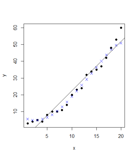
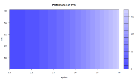
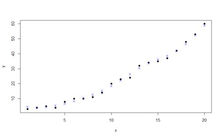
 SVM
SVM