This represents Part 2 of a 4-part series relative to the calculation of Equity Cash Flow (ECF) using R. If you missed Part 1, be certain read that first part before proceeding. The content builds off prior described information/data. Part 1 previous post is located here.
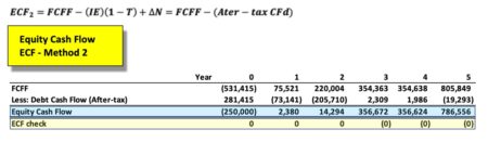
‘ECF – Method 2’ is defined as follows:
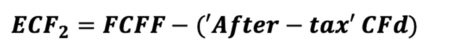 The equation appears innocent enough, though there are many underlying terms that require definition for understanding of the calculation. In words, ‘ECF – Method 2’ equals free cash Flow (FCFF) minus after-tax Debt Cash Flow (CFd).
Reference details of the 5-year capital project’s fully integrated financial statements developed in R at the following link. The R output is formatted in Excel. Zoom for detail.
https://www.dropbox.com/s/lx3uz2mnei3obbb/financial_statements.pdf?dl=0
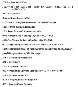
The first order of business is to define the terms necessary to calculate FCFF.
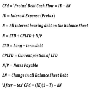
Next, pretax Debt Cash Flow (CFd) and its components are defined as follows:
data <- data %>%
  mutate(ie    = c(0, 10694, 8158, 527, 627, 717 ),
         np    = c(31415, 9188, 13875,  16500, 18863, 0),
         LTD   = c(250000, 184952, 0, 0, 0, 0),
         cpltd = c(0, 20550, 0, 0, 0, 0),
         ni    =  c(0, 47584,  141355,  262035, 325894, 511852),
         bd    =  c(0, 62500,  62500,   62500,   62500,   62500),
         chg_DTL_net = c(0, 35000,  55000,  35000, -25000, -100000),
         cash  = c(30500,  61250, 92500, 110000, 125750, 0),
         ar    = c(0, 61250,  92500,  110000,  125750, 0),
         inv   = c(30500, 61250, 92500, 110000,  125750, 0),
         pe    = c(915, 1838, 2775, 3300, 3773, 0),
         ap    = c(30500, 73500, 111000, 132000, 150900, 0),
         wp    = c(0, 5513, 8325, 9900, 11318, 0),
         itp   = c(0, -819.377,  9809,  34923, 60566, 0),
         CapX  = c(500000,0,0,0,0,0),
         gain  = c(0,0,0,0,0,162500),
         sp  = c(0,0,0,0,0,350000))
View tibble.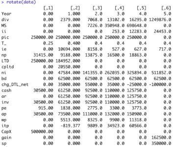
All of the above calculations are defined in the below R function ECF_2. ‘ECF – Method 2’ R function
ECF_2 <- function(a) {

  ECF2 <-      tibble(T_        = a$T_,
                       ie       = a$ie,
                       ii       = a$ii,
                       Year     = c(0:(length(ii)-1)),
                       ni       = a$ni,
                       bd       = a$bd,
                       chg_DTL_net = a$chg_DTL_net,
                       gain     = - a$gain,
                       sp       = a$sp,
                       ie_AT    = ie*(1-a$T_),
                       ii_AT    = - ii*(1-a$T_),
                       gcf      = ni + bd + chg_DTL_net + gain + sp
                                + ie_AT + ii_AT,
                       OCA      = a$cash + a$ar + a$inv + a$pe,
                       OCL      = a$ap + a$wp + a$itp,
                       OWC      = OCA - OCL,
                       chg_OWC  = OWC - lag(OWC, default=0),
                       CapX     = - a$CapX,
                       FCFF1    = gcf + CapX - chg_OWC,
                       N        = a$LTD + a$cpltd + a$np,
                       chg_N    = N - lag(N, default=0),
                       CFd_AT   = ie*(1-T_) - chg_N,
                       ECF2     = FCFF1 - CFd_AT )


  ECF2 <- rotate(ECF2)
  return(ECF2)

}
Run the R function and view the output.
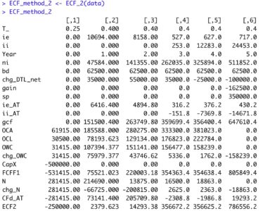
R Output formatted in Excel Method 2
‘ECF Method 2‘ agrees with the prior results from ‘ECF Method 1‘ each year. Any differences are due to rounding error.
This ECF calculation example is taken from my newly published textbook, ‘Advanced Discounted Cash Flow (DCF) Valuation using R.’ It is discussed in far greater detail along with development of the integrated financials using R as well as numerous, advanced DCF valuation modeling approaches – some never before published. The text importantly clearly explains ‘why’ these ECF calculation methods are mathematically exactly equivalent, though the individual components appear vastly different.
Reference my website for further details.
https://www.leewacc.com/
Next up, ‘ECF – Method 3’ …
Brian K. Lee, MBA, PRM, CMA, CFA