Over the next several days, I will present 4 different methods of correctly calculating Equity Cash Flow (ECF) using R. The valuation technique of discounted cash flow (DCF) estimates equity value (E) as the present value of forecasted ECF. The appropriate discount rate for this flow definition is the cost of equity capital (Ke).
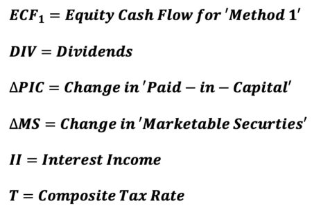
‘ECF – Method 1’ is defined as follows:
where

Note: ECF is not simply ‘dividends.’ A common misconception is that discounted dividends (DIV) provide equity value. An example of this is the common ‘dividend growth’ equity valuation model found in many corporate finance texts. All ‘dividend growth’ models that discount dividends (DIV) at the cost of equity capital (Ke) are incorrect unless forecasted 1) marketable securities (MS) balances are zero, and 2) there is no issuance or repurchase of equity shares.
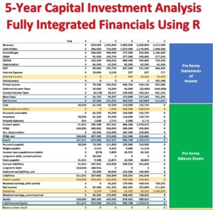
The data assumes a 5-year year hypothetical capital project. A single revenue producing asset is purchased at the end of ‘Year 0‘ and is sold at the end of ‘Year 5.’ The $500,000 asset is purchased assuming 50% debt and 50% equity financing.
Further, the data used to estimate ECF in this example are taken from fully integrated pro forma financial statements and other relevant data assumptions including the corporate tax rate. This particular example only requires financial data from integrated pro forma income statements and balance sheets. These 2 pro forma financial statements are shown below with the relevant data rows highlighted.

https://www.dropbox.com/s/xwy97flxe99gqr9/financials.pdf?dl=0
The above link provides access to a PDF of all financial statement pro forma data and is easily zoomable for viewing purposes.
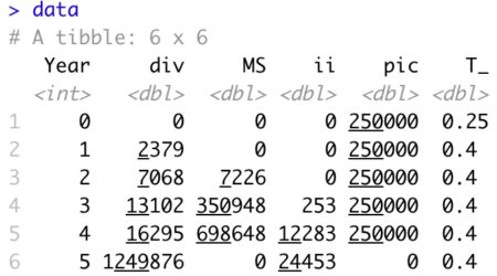
The relevant data used to calculate ECF are initially placed in a tibble.
library(tidyverse)


data <- tibble(Year = c(0:5),
              div  = c(0, 2379, 7068, 13102, 16295, 1249876),
              MS   = c(0, 0, 7226, 350948, 698648, 0),
              ii   = c(0, 0, 0, 253, 12283, 24453),
              pic  = c(250000, 250000, 250000, 250000, 250000, 0),
              T_   = c(0.25, 0.40, 0.40, 0.40, 0.40, 0.40))

data

An R function is created to rotate the data in standard financial data presentation format (each data line item occupies a single row instead of a column)
rotate <- function(r) {

  p <- t(as.matrix(as_tibble(r)))

  return(p)

}
View the rotated data.
rotate(data)

An R function reads in the appropriate data, performs the necessary calculations, and outputs the data. The R output is then placed in a spreadsheet to formatting purposes.
‘ECF – Method 1’ R function
ECF_1 <- function(a) {

  ECF1 <-     tibble( T_             = a$T_,
                      pic            = a$pic,
                      chg_pic        = pic - lag(pic, default=0),
                      MS             = a$MS,
                      ii             = a$ii,
                      Year           = c(0:(length(T_)-1)),
                      div            = a$div,
                      net_new_equity = -chg_pic,
                      chg_MS         = MS - lag(MS, default=0),
                      ii_AT          = -ii*(1-T_),
                      ECF1           = div + net_new_equity
                                       + chg_MS + ii_AT )

  ECF1 <- rotate(ECF1)

  return(ECF1)

}
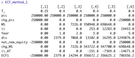
View R Output
ECF_method_1 <- ECF_1( data)
ECF_method_1

Excel formatting applied to R Output

It is quite evident there is far more than just dividends (DIV) involved in the proper calculation of ECF. Use of a ‘dividend growth’ equity valuation model in this instance would result in significant model error.
This ECF calculation example is taken from my newly published textbook, ‘Advanced Discounted Cash Flow (DCF) Valuation using R.’ It is discussed in far greater detail along with development of the integrated financials using R as well as numerous, advanced DCF valuation modeling approaches – some never before published.
Reference my website for further details.
https://www.leewacc.com/
Next up, ‘ECF – Method 2’ …
Brian K. Lee, MBA, PRM, CMA, CFA