ROC for Decision Trees – where did the data come from?
By Jerry Tuttle
In doing decision tree classification problems, I have often graphed the ROC (Receiver Operating Characteristic) curve. The True Positive Rate (TPR) is on the y-axis, and the False Positive Rate (FPR) is on the x-axis. True Positive is when the lab test predicts you have the disease and you actually do have it. False Positive is when the lab test predicts you have the disease but you actually do not have it.
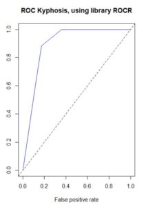
The following code uses the sample dataset kyphosis from the rpart package, creates a default decision tree, prints the confusion matrix, and plots the ROC curve. (Kyphosis is a type of spinal deformity.)
library(rpart)
df <- kyphosis
set.seed(1)
mytree <- rpart(Kyphosis ~ Age + Number + Start, data = df, method="class")
library(rattle)
library(rpart.plot)
library(RColorBrewer)
fancyRpartPlot(mytree, uniform=TRUE, main="Kyphosis Tree")
predicted <- predict(mytree, type="class")
table(df$Kyphosis,predicted)
library(ROCR)
pred <- prediction(predict(mytree, type="prob")[, 2], df$Kyphosis)
plot(performance(pred, "tpr", "fpr"), col="blue", main="ROC Kyphosis, using library ROCR")
abline(0, 1, lty=2)
auc <- performance(pred, "auc")
auc@y.values

However, for a long time there has been a disconnect in my mind between the confusion matrix and the ROC curve. The confusion matrix provides a single value of the ordered pair (x=FPR, y=TPR) on the ROC curve, but the ROC curve has a range of values. Where are the other values coming from?
The answer is that a default decision tree confusion matrix uses a single probability threshold value of 50%. A decision tree ends in a set of terminal nodes. Every observation falls in exactly one of those terminal nodes. The predicted classification for the entire node is based on whichever classification has the greater percentage of observations, which for binary classifications requires a probability greater than 50%. So for example if a single observation has predicted probability based on its terminal node of 58% that the disease is present, then a 50% threshold would classify this observation as disease being present. But if the threshold were changed to 60%, then the observation would be classified as disease not being present.
The ROC curve uses a variety of probability thresholds, reclassifies each observation, recalculates the confusion matrix, and recalculates a new value of the ordered pair (x=FPR, y=TPR) for the ROC curve. The resulting curve shows the spread of these ordered pairs over all (including interpolated, and possibly extrapolated) probability thresholds, but the threshold values are not commonly displayed on the curve. Plotting performance in the ROCR package does this behind the scenes, but I wanted to verify this myself. This dataset has a small number of predictions of disease present, and at large threshold values the prediction is zero, resulting in a one column confusion matrix and zero FPR and TPR. The following code individually applies different probability thresholds to build the ROC curve, although it does not extrapolate for large values of FPR and TPR.
dat <- data.frame()
s <- predict(mytree, type="prob")[, 2]
for (i in 1:21){
p <- .05*(i-1)
thresh p, “present”, “absent”)
t <- table(df$Kyphosis,thresh)
fpr <- ifelse(ncol(t)==1, 0, t[1,2] / (t[1,2] + t[1,1]))
tpr <- ifelse(ncol(t)==1, 0, t[2,2] / (t[2,2] + t[2,1]))
dat[i,1] <- fpr
dat[i,2] <- tpr
}
colnames(dat) <- c("fpr", "tpr")
plot(x=dat$fpr, y=dat$tpr, xlab="FPR", ylab="TPR", xlim=c(0,1), ylim=c(0,1),
main="ROC Kyphosis, using indiv threshold calcs", type="b", col="blue")
abline(0, 1, lty=2)