Support Vector Machines (SVM) is a data classification method that separates data using hyperplanes. The concept of SVM is very intuitive and easily understandable. If we have labeled data, SVM can be used to generate multiple separating hyperplanes such that the data space is divided into segments and each segment contains only one kind of data. SVM technique is generally useful for data which has non-regularity which means, data whose distribution is unknown. Let’s take a simple example to understand how SVM works. Say you have only two kinds of values and we can represent them as in the figure:
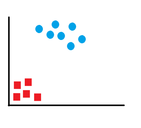 This data is simple to classify and one can see that the data is clearly separated into two segments. Any line that separates the red and blue items can be used to classify the above data. Had this data been multi-dimensional data, any plane can separate and successfully classify the data. However, we want to find the “most optimal” solution. What will then be the characteristic of this most optimal line? We have to remember that this is just the training data and we can have more data points which can lie anywhere in the subspace. If our line is too close to any of the datapoints, noisy test data is more likely to get classified in a wrong segment. We have to choose the line which lies between these groups and is at the farthest distance from each of the segments.
To solve this classifier line, we draw the line as y=ax+b and make it equidistant from the respective data points closest to the line. So we want to maximize the margin (m).
This data is simple to classify and one can see that the data is clearly separated into two segments. Any line that separates the red and blue items can be used to classify the above data. Had this data been multi-dimensional data, any plane can separate and successfully classify the data. However, we want to find the “most optimal” solution. What will then be the characteristic of this most optimal line? We have to remember that this is just the training data and we can have more data points which can lie anywhere in the subspace. If our line is too close to any of the datapoints, noisy test data is more likely to get classified in a wrong segment. We have to choose the line which lies between these groups and is at the farthest distance from each of the segments.
To solve this classifier line, we draw the line as y=ax+b and make it equidistant from the respective data points closest to the line. So we want to maximize the margin (m).
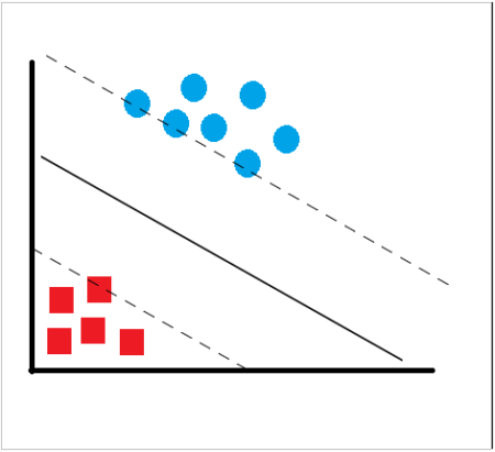 We know that all points on the line ax+b=0 will satisfy the equation. If we draw two parallel lines – ax+b=-1 for one segment and ax+b=1 for the other segment such that these lines pass through a datapoint in the segment which is nearest to our line then the distance between these two lines will be our margin. Hence, our margin will be m=2/||a||. Looked at another way, if we have a training dataset (x1,x2,x3…xn) and want to produce and outcome y such that y is either -1 or 1 (depending on which segment the datapoint belongs to), then our classifier should correctly classify data points in the form of y=ax+b. This also means that y(ax+b)>1 for all data points. Since we have to maximize the margin, we have the solve this problem with the constraint of maximizing 2/||a|| or, minimizing ||a||^2/2 which is basically the dual form of the constraint. Solving this can be easy or complex depending upon the dimensionality of data. However, we can do this quickly with R and try out with some sample dataset.
To use SVM in R, I just created a random data with two features x and y in excel. I took all the values of x as just a sequence from 1 to 20 and the corresponding values of y as derived using the formula y(t)=y(t-1) + r(-1:9) where r(a,b) generates a random integer between a and b. I took y(1) as 3. The following code in R illustrates a set of sample generated values:
x=c(1,2,3,4,5,6,7,8,9,10,11,12,13,14,15,16,17,18,19,20)
y=c(3,4,5,4,8,10,10,11,14,20,23,24,32,34,35,37,42,48,53,60)
#Create a data frame of the data
train=data.frame(x,y)
Let’s see how our data looks like. For this we use the plot function
#Plot the dataset
plot(train,pch=16)
We know that all points on the line ax+b=0 will satisfy the equation. If we draw two parallel lines – ax+b=-1 for one segment and ax+b=1 for the other segment such that these lines pass through a datapoint in the segment which is nearest to our line then the distance between these two lines will be our margin. Hence, our margin will be m=2/||a||. Looked at another way, if we have a training dataset (x1,x2,x3…xn) and want to produce and outcome y such that y is either -1 or 1 (depending on which segment the datapoint belongs to), then our classifier should correctly classify data points in the form of y=ax+b. This also means that y(ax+b)>1 for all data points. Since we have to maximize the margin, we have the solve this problem with the constraint of maximizing 2/||a|| or, minimizing ||a||^2/2 which is basically the dual form of the constraint. Solving this can be easy or complex depending upon the dimensionality of data. However, we can do this quickly with R and try out with some sample dataset.
To use SVM in R, I just created a random data with two features x and y in excel. I took all the values of x as just a sequence from 1 to 20 and the corresponding values of y as derived using the formula y(t)=y(t-1) + r(-1:9) where r(a,b) generates a random integer between a and b. I took y(1) as 3. The following code in R illustrates a set of sample generated values:
x=c(1,2,3,4,5,6,7,8,9,10,11,12,13,14,15,16,17,18,19,20)
y=c(3,4,5,4,8,10,10,11,14,20,23,24,32,34,35,37,42,48,53,60)
#Create a data frame of the data
train=data.frame(x,y)
Let’s see how our data looks like. For this we use the plot function
#Plot the dataset
plot(train,pch=16)
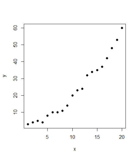
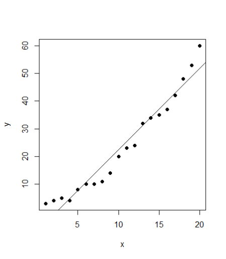
Seems to be a fairly good data. Looking at the plot, it also seems like a linear regression should also be a good fit to the data. We’ll use both the models and compare them. First, the code for linear regression: #Linear regression model <- lm(y ~ x, train) #Plot the model using abline abline(model)
 SVM
To use SVM in R, we have a package e1071. The package is not preinstalled, hence one needs to run the line “install.packages(“e1071”) to install the package and then import the package contents using the library command. The syntax of svm package is quite similar to linear regression. We use svm function here.
#SVM
library(e1071)
#Fit a model. The function syntax is very similar to lm function
model_svm <- svm(y ~ x , train)
#Use the predictions on the data
pred <- predict(model_svm, train)
#Plot the predictions and the plot to see our model fit
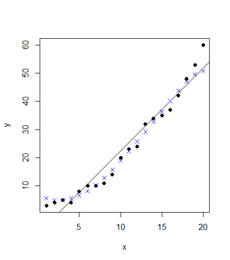
points(train$x, pred, col = "blue", pch=4)
SVM
To use SVM in R, we have a package e1071. The package is not preinstalled, hence one needs to run the line “install.packages(“e1071”) to install the package and then import the package contents using the library command. The syntax of svm package is quite similar to linear regression. We use svm function here.
#SVM
library(e1071)
#Fit a model. The function syntax is very similar to lm function
model_svm <- svm(y ~ x , train)
#Use the predictions on the data
pred <- predict(model_svm, train)
#Plot the predictions and the plot to see our model fit
points(train$x, pred, col = "blue", pch=4)
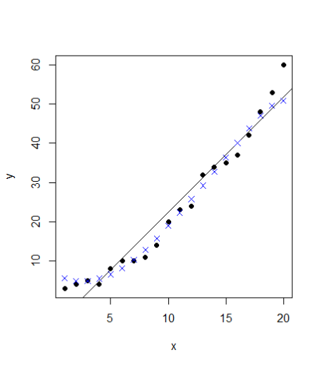 The points follow the actual values much more closely than the abline. Can we verify that? Let’s calculate the rmse errors for both the models:
#Linear model has a residuals part which we can extract and directly calculate rmse
error <- model$residuals
lm_error <- sqrt(mean(error^2)) # 3.832974
#For svm, we have to manually calculate the difference between actual values (train$y) with our predictions (pred)
error_2 <- train$y – pred
svm_error <- sqrt(mean(error_2^2)) &amp;amp;amp;amp;nbsp;# 2.696281
In this case, the rmse for linear model is ~3.83 whereas our svm model has a lower error of ~2.7. A straightforward implementation of SVM has an accuracy higher than the linear regression model. However, the SVM model goes far beyond that. We can further improve our SVM model and tune it so that the error is even lower. We will now go deeper into the SVM function and the tune function. We can specify the values for the cost parameter and epsilon which is 0.1 by default. A simple way is to try for each value of epsilon between 0 and 1 (I will take steps of 0.01) and similarly try for cost function from 4 to 2^9 (I will take exponential steps of 2 here). I am taking 101 values of epsilon and 8 values of cost function. I will thus be testing 808 models and see which ones performs best. The code may take a short while to run all the models and find the best version. The corresponding code will be
svm_tune <- tune(svm, y ~ x, &amp;amp;amp;amp;nbsp;data = train,
ranges = list(epsilon = seq(0,1,0.01), cost = 2^(2:9))
)
print(svm_tune)
#Printing gives the output:
#Parameter tuning of ‘svm’:
# – sampling method: 10-fold cross validation
#- best parameters:
# epsilon cost
#0.09 256
#- best performance: 2.569451
#This best performance denotes the MSE. The corresponding RMSE is 1.602951 which is square root of MSE
An advantage of tuning in R is that it lets us extract the best function directly. We don’t have to do anything and just extract the best function from the svm_tune list. We can now see the improvement in our model by calculating its RMSE error using the following code
#The best model
best_mod <- svm_tune$best.model
best_mod_pred <- predict(best_mod, train)
error_best_mod <- train$y – best_mod_pred
# this value can be different on your computer
# because the tune method randomly shuffles the data
best_mod_RMSE <- sqrt(mean(error_best_mod^2)) # 1.290738
This tuning method is known as grid search. R runs all various models with all the possible values of epsilon and cost function in the specified range and gives us the model which has the lowest error. We can also plot our tuning model to see the performance of all the models together
plot(svm_tune)
The points follow the actual values much more closely than the abline. Can we verify that? Let’s calculate the rmse errors for both the models:
#Linear model has a residuals part which we can extract and directly calculate rmse
error <- model$residuals
lm_error <- sqrt(mean(error^2)) # 3.832974
#For svm, we have to manually calculate the difference between actual values (train$y) with our predictions (pred)
error_2 <- train$y – pred
svm_error <- sqrt(mean(error_2^2)) &amp;amp;amp;amp;nbsp;# 2.696281
In this case, the rmse for linear model is ~3.83 whereas our svm model has a lower error of ~2.7. A straightforward implementation of SVM has an accuracy higher than the linear regression model. However, the SVM model goes far beyond that. We can further improve our SVM model and tune it so that the error is even lower. We will now go deeper into the SVM function and the tune function. We can specify the values for the cost parameter and epsilon which is 0.1 by default. A simple way is to try for each value of epsilon between 0 and 1 (I will take steps of 0.01) and similarly try for cost function from 4 to 2^9 (I will take exponential steps of 2 here). I am taking 101 values of epsilon and 8 values of cost function. I will thus be testing 808 models and see which ones performs best. The code may take a short while to run all the models and find the best version. The corresponding code will be
svm_tune <- tune(svm, y ~ x, &amp;amp;amp;amp;nbsp;data = train,
ranges = list(epsilon = seq(0,1,0.01), cost = 2^(2:9))
)
print(svm_tune)
#Printing gives the output:
#Parameter tuning of ‘svm’:
# – sampling method: 10-fold cross validation
#- best parameters:
# epsilon cost
#0.09 256
#- best performance: 2.569451
#This best performance denotes the MSE. The corresponding RMSE is 1.602951 which is square root of MSE
An advantage of tuning in R is that it lets us extract the best function directly. We don’t have to do anything and just extract the best function from the svm_tune list. We can now see the improvement in our model by calculating its RMSE error using the following code
#The best model
best_mod <- svm_tune$best.model
best_mod_pred <- predict(best_mod, train)
error_best_mod <- train$y – best_mod_pred
# this value can be different on your computer
# because the tune method randomly shuffles the data
best_mod_RMSE <- sqrt(mean(error_best_mod^2)) # 1.290738
This tuning method is known as grid search. R runs all various models with all the possible values of epsilon and cost function in the specified range and gives us the model which has the lowest error. We can also plot our tuning model to see the performance of all the models together
plot(svm_tune)
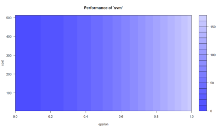 This plot shows the performance of various models using color coding. Darker regions imply better accuracy. The use of this plot is to determine the possible range where we can narrow down our search to and try further tuning if required. For instance, this plot shows that I can run tuning for epsilon in the new range of 0 to 0.2 and while I’m at it, I can move in even lower steps (say 0.002) but going further may lead to overfitting so I can stop at this point. From this model, we have improved on our initial error of 2.69 and come as close as 1.29 which is about half of our original error in SVM. We have come very far in our model accuracy. Let’s see how the best model looks like when plotted.
plot(train,pch=16)
points(train$x, best_mod_pred, col = "blue", pch=4)
This plot shows the performance of various models using color coding. Darker regions imply better accuracy. The use of this plot is to determine the possible range where we can narrow down our search to and try further tuning if required. For instance, this plot shows that I can run tuning for epsilon in the new range of 0 to 0.2 and while I’m at it, I can move in even lower steps (say 0.002) but going further may lead to overfitting so I can stop at this point. From this model, we have improved on our initial error of 2.69 and come as close as 1.29 which is about half of our original error in SVM. We have come very far in our model accuracy. Let’s see how the best model looks like when plotted.
plot(train,pch=16)
points(train$x, best_mod_pred, col = "blue", pch=4)
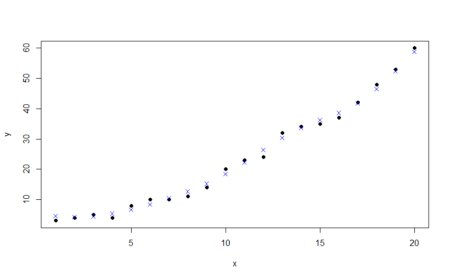 Visually, the points predicted by our tuned model almost follow the data. This is the power of SVM and we are just seeing this for data with two features. Imagine the abilities of the model with more number of complex features!
Summary
SVM is a powerful technique and especially useful for data whose distribution is unknown (also known as non-regularity in data). Because the example considered here consisted of only two features, the SVM fitted by R here is also known as linear SVM. SVM is powered by a kernel for dealing with various kinds of data and its kernel can also be set during model tuning. Some such examples include gaussian and radial. Hence, SVM can also be used for non-linear data and does not require any assumptions about its functional form. Because we separate data with the maximum possible margin, the model becomes very robust and can deal with incongruencies such as noisy test data or biased train data. We can also interpret the results produced by SVM through visualization. A common disadvantage with SVM is associated with its tuning. The level of accuracy in predicting over the training data has to be defined in our data. Because our example was custom generated data, we went ahead and tried to get our model accuracy as high as possible by reducing the error. However, in business situations when one needs to train the model and continually predict over test data, SVM may fall into the trap of overfitting. This is the reason SVM needs to be carefully modeled – otherwise the model accuracy may not be satisfactory. As I did in the example, SVM technique is closely related to regression technique. For linear data, we can compare SVM with linear regression while non-linear SVM is comparable to logistic regression. As the data becomes more and more linear in nature, linear regression becomes more and more accurate. At the same time, tuned SVM can also fit the data. However, noisiness and bias can severely impact the ability of regression. In such cases, SVM comes in really handy!
With this article, I hope one may understand the basics of SVM and its implementation in R. One can also deep dive into the SVM technique by using model tuning. The full R code used in the article is laid out as under:
x=c(1,2,3,4,5,6,7,8,9,10,11,12,13,14,15,16,17,18,19,20)
y=c(3,4,5,4,8,10,10,11,14,20,23,24,32,34,35,37,42,48,53,60)
#Create a data frame of the data
train=data.frame(x,y)
#Plot the dataset
plot(train,pch=16)
#Linear regression
model <- lm(y ~ x, train)
#Plot the model using abline
abline(model)
#SVM
library(e1071)
#Fit a model. The function syntax is very similar to lm function
model_svm <- svm(y ~ x , train)
#Use the predictions on the data
pred <- predict(model_svm, train)
#Plot the predictions and the plot to see our model fit
points(train$x, pred, col = "blue", pch=4)
#Linear model has a residuals part which we can extract and directly calculate rmse
error <- model$residuals
lm_error <- sqrt(mean(error^2)) # 3.832974
#For svm, we have to manually calculate the difference between actual values (train$y) with our predictions (pred)
error_2 <- train$y – pred
svm_error <- sqrt(mean(error_2^2)) # 2.696281
# perform a grid search
svm_tune <- tune(svm, y ~ x, data = train,
ranges = list(epsilon = seq(0,1,0.01), cost = 2^(2:9))
)
print(svm_tune)
#Parameter tuning of ‘svm’:
# – sampling method: 10-fold cross validation
#- best parameters:
# epsilon cost
#0 8
#- best performance: 2.872047
#The best model
best_mod <- svm_tune$best.model
best_mod_pred <- predict(best_mod, train)
error_best_mod <- train$y – best_mod_pred
# this value can be different on your computer
# because the tune method randomly shuffles the data
best_mod_RMSE <- sqrt(mean(error_best_mod^2)) # 1.290738
plot(svm_tune)
plot(train,pch=16)
points(train$x, best_mod_pred, col = "blue", pch=4)
Bio: Chaitanya Sagar is the Founder and CEO of Perceptive Analytics. Perceptive Analytics has been chosen as one of the top 10 analytics companies to watch out for by Analytics India Magazine. It works on Marketing Analytics for e-commerce, Retail and Pharma companies.
Visually, the points predicted by our tuned model almost follow the data. This is the power of SVM and we are just seeing this for data with two features. Imagine the abilities of the model with more number of complex features!
Summary
SVM is a powerful technique and especially useful for data whose distribution is unknown (also known as non-regularity in data). Because the example considered here consisted of only two features, the SVM fitted by R here is also known as linear SVM. SVM is powered by a kernel for dealing with various kinds of data and its kernel can also be set during model tuning. Some such examples include gaussian and radial. Hence, SVM can also be used for non-linear data and does not require any assumptions about its functional form. Because we separate data with the maximum possible margin, the model becomes very robust and can deal with incongruencies such as noisy test data or biased train data. We can also interpret the results produced by SVM through visualization. A common disadvantage with SVM is associated with its tuning. The level of accuracy in predicting over the training data has to be defined in our data. Because our example was custom generated data, we went ahead and tried to get our model accuracy as high as possible by reducing the error. However, in business situations when one needs to train the model and continually predict over test data, SVM may fall into the trap of overfitting. This is the reason SVM needs to be carefully modeled – otherwise the model accuracy may not be satisfactory. As I did in the example, SVM technique is closely related to regression technique. For linear data, we can compare SVM with linear regression while non-linear SVM is comparable to logistic regression. As the data becomes more and more linear in nature, linear regression becomes more and more accurate. At the same time, tuned SVM can also fit the data. However, noisiness and bias can severely impact the ability of regression. In such cases, SVM comes in really handy!
With this article, I hope one may understand the basics of SVM and its implementation in R. One can also deep dive into the SVM technique by using model tuning. The full R code used in the article is laid out as under:
x=c(1,2,3,4,5,6,7,8,9,10,11,12,13,14,15,16,17,18,19,20)
y=c(3,4,5,4,8,10,10,11,14,20,23,24,32,34,35,37,42,48,53,60)
#Create a data frame of the data
train=data.frame(x,y)
#Plot the dataset
plot(train,pch=16)
#Linear regression
model <- lm(y ~ x, train)
#Plot the model using abline
abline(model)
#SVM
library(e1071)
#Fit a model. The function syntax is very similar to lm function
model_svm <- svm(y ~ x , train)
#Use the predictions on the data
pred <- predict(model_svm, train)
#Plot the predictions and the plot to see our model fit
points(train$x, pred, col = "blue", pch=4)
#Linear model has a residuals part which we can extract and directly calculate rmse
error <- model$residuals
lm_error <- sqrt(mean(error^2)) # 3.832974
#For svm, we have to manually calculate the difference between actual values (train$y) with our predictions (pred)
error_2 <- train$y – pred
svm_error <- sqrt(mean(error_2^2)) # 2.696281
# perform a grid search
svm_tune <- tune(svm, y ~ x, data = train,
ranges = list(epsilon = seq(0,1,0.01), cost = 2^(2:9))
)
print(svm_tune)
#Parameter tuning of ‘svm’:
# – sampling method: 10-fold cross validation
#- best parameters:
# epsilon cost
#0 8
#- best performance: 2.872047
#The best model
best_mod <- svm_tune$best.model
best_mod_pred <- predict(best_mod, train)
error_best_mod <- train$y – best_mod_pred
# this value can be different on your computer
# because the tune method randomly shuffles the data
best_mod_RMSE <- sqrt(mean(error_best_mod^2)) # 1.290738
plot(svm_tune)
plot(train,pch=16)
points(train$x, best_mod_pred, col = "blue", pch=4)
Bio: Chaitanya Sagar is the Founder and CEO of Perceptive Analytics. Perceptive Analytics has been chosen as one of the top 10 analytics companies to watch out for by Analytics India Magazine. It works on Marketing Analytics for e-commerce, Retail and Pharma companies.
Bravo guys! loved this article.. I am a XGboost lover but I’ve had some problems tuning it with iterations like you just explained here! Great stuff..
The closing parentheses (“)”) is missing in the sum_tune statement