It can be easy to explore data generating mechanisms with the simstudy package

Interested in publishing a one-time post on R-bloggers.com? Press here to learn how.

---

I learned statistics and probability by simulating data. Sure, I battled my way through proofs, but I never believed the results until I saw it in a simulation. I guess I have it backwards, it worked for me. And now that I do this for a living, I continue to use simulation to understand models, to do sample size estimates and power calculations, and of course to teach. Sure – I’ll use the occasional formula, but I always feel the need to check it with simulation. It’s just the way I am.

Since I found myself constantly setting up simulations, over time I developed ways to make the process a bit easier. Those processes turned into a package, which I called simstudy, or simulating study data. My goal here is to introduce the basic idea behind simstudy, and provide a relatively simple example that comes from a question posed by a user who was trying to generate correlated longitudinal data.

The basic idea

Simulation using simstudy has two essential steps. First, the user defines the data elements of a data set either in an external csv file or internally through a set of repeated definition statements. Second, the user generates the data, using these definitions. Data generation can be as simple as a cross-sectional design or prospective cohort design, or it can be more involved. Simulation can include observed or randomized treatment assignment/exposures, survival data, longitudinal/panel data, multi-level/hierarchical data, data sets with correlated variables based on a specified covariance structure, and data sets with missing data resulting from any sort of missingness pattern.

The key to simulating data in simstudy is the creation of series of data definition tables that look like this: 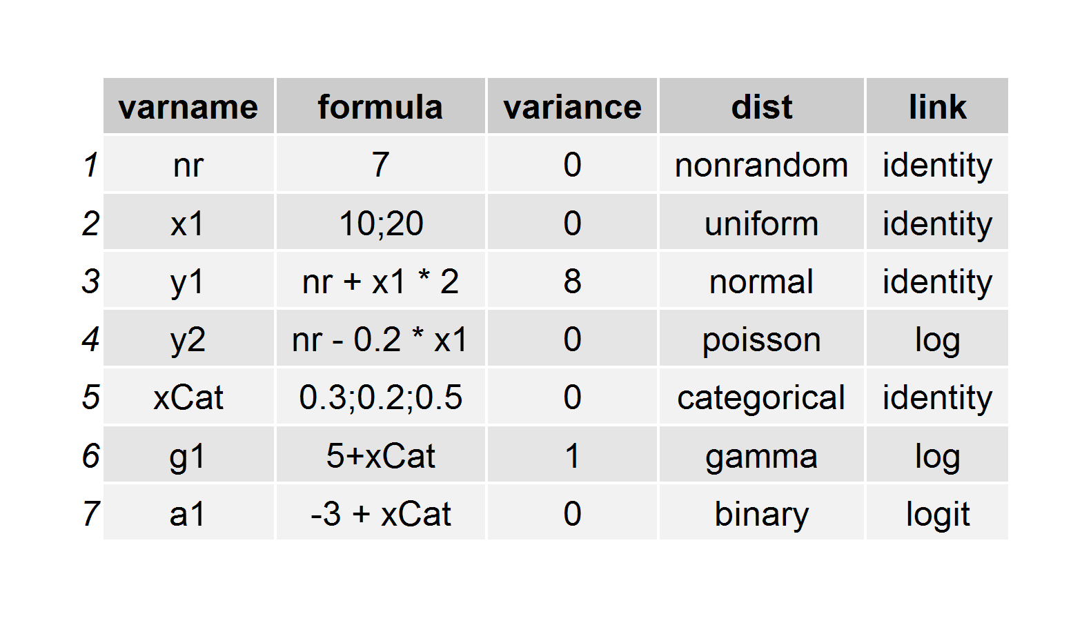Here’s the code that is used to generate this definition, which is stored as a data.table :

def <- defData(varname = "nr", dist = "nonrandom", formula = 7, id = "idnum")
def <- defData(def, varname = "x1", dist = "uniform", formula = "10;20")
def <- defData(def, varname = "y1", formula = "nr + x1 * 2", variance = 8)
def <- defData(def, varname = "y2", dist = "poisson", formula = "nr - 0.2 * x1", link = "log")
def <- defData(def, varname = "xCat", formula = "0.3;0.2;0.5", dist = "categorical")
def <- defData(def, varname = "g1", dist = "gamma", formula = "5+xCat", variance = 1, link = "log")
def <- defData(def, varname = "a1", dist = "binary", formula = "-3 + xCat", link = "logit")

To create a simple data set based on these definitions, all one needs to do is execute a single genData command. In this example, we generate 500 records that are based on the definition in the def table:

dt <- genData(500, def)

dt

[code language="lang="r"]
##      idnum nr       x1       y1  y2 xCat          g1 a1
##   1:     1  7 10.74929 30.01273 123    3 13310.84731  0
##   2:     2  7 18.56196 44.77329  17    1   395.41606  0
##   3:     3  7 16.96044 43.76427  42    3   522.45258  0
##   4:     4  7 19.51511 45.14214  22    3  3045.06826  0
##   5:     5  7 10.79791 27.25012 128    1   406.88647  0
##  ---                                                   
## 496:   496  7 19.96636 52.05377  21    3   264.85557  1
## 497:   497  7 15.97957 39.62428  44    2    40.59823  0
## 498:   498  7 19.74036 47.32292  21    3  3410.54787  0
## 499:   499  7 19.71597 48.26259  25    3   206.90961  1
## 500:   500  7 14.60405 28.94185  53    1    97.43068  0

There’s a lot more functionality in the package, and I’ll be writing about that in the future. But here, I just want give a little more introduction by way of an example that came in from across the globe a couple of days ago. (I’d say the best thing about building an R package is hearing from folks literally all over the world and getting to talk to them about statistics and R.)

Going a bit further: simulating a prospective cohort study with repeated measures

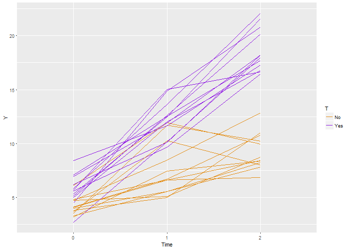
The question was, can we simulate a study with two arms, say a control and treatment, with repeated measures at three time points: baseline, after 1 month, and after 2 months? The answer is, of course.

Drawing on her original code, we wanted a scenario the included two treatment arms or exposures and three measurements per individual. The change over time was supposed to be greater for one of the groups. This was what I sent back to my correspondent:

# Define the outcome

ydef <- defDataAdd(varname = "Y", dist = "normal", 
                   formula = "5 + 2.5*period + 1.5*T + 3.5*period*T", 
                   variance = 3)

# Generate a 'blank' data.table with 24 observations and assign them to groups

set.seed(1234)

indData <- genData(24)
indData <- trtAssign(indData, nTrt = 2, balanced = TRUE, grpName = "T")

# Create a longitudinal data set of 3 records for each id

longData <- addPeriods(indData, nPeriods = 3, idvars = "id")
longData <- addColumns(dtDefs = ydef, longData)

longData[, `:=`(T, factor(T, labels = c("No", "Yes")))]

# Let's look at the data

ggplot(data = longData, aes(x = factor(period), y = Y)) + geom_line(aes(color = T, 
    group = id)) + scale_color_manual(values = c("#e38e17", "#8e17e3")) + xlab("Time")

My correspondent quickly pointed out that I hadn’t really provided her with the full solution – as the measurements for each individual in the example above are not correlated across the time periods. If we generate a data set based on 1,000 individuals and estimate a linear regression model we see that the parameter estimates are quite good, though we can see from the estimate of alpha (at the bottom of the output), which was approximately 0.02, that there is little within-individual correlation:

# Fit a GEE model to the data

fit <- geeglm(Y ~ factor(T) + period + factor(T) * period, family = gaussian(link = "identity"), 
    data = longData, id = id, corstr = "exchangeable")
summary(fit)

## 
## Call:
## geeglm(formula = Y ~ factor(T) + period + factor(T) * period, 
##     family = gaussian(link = "identity"), data = longData, id = id, 
##     corstr = "exchangeable")
## 
##  Coefficients:
##                     Estimate Std.err   Wald Pr(>|W|)    
## (Intercept)          4.98268 0.07227 4753.4   <2e-16 ***
## factor(T)Yes         1.48555 0.10059  218.1   <2e-16 ***
## period               2.53946 0.05257 2333.7   <2e-16 ***
## factor(T)Yes:period  3.51294 0.07673 2096.2   <2e-16 ***
## ---
## Signif. codes:  0 '***' 0.001 '**' 0.01 '*' 0.05 '.' 0.1 ' ' 1
## 
## Estimated Scale Parameters:
##             Estimate Std.err
## (Intercept)    2.952 0.07325
## 
## Correlation: Structure = exchangeable  Link = identity 
## 
## Estimated Correlation Parameters:
##       Estimate Std.err
## alpha  0.01737 0.01862
## Number of clusters:   1000   Maximum cluster size: 3

One way to generate correlated data

To address this shortcoming, there are at least two ways we can go about it. The first is to use the simstudy function genCorData. In this example, we generate correlated errors that are normally distributed with mean 0, variance 3, and common correlation coefficient of 0.7. Using this approach, the underlying data generation process is a bit cryptic, because we are acknowledging that we don’t know what is driving the relationship between the three outcomes, just that they have some common cause or other relationship that results in a strong relationship. However, it does the trick:

# define the outcome
ydef <- defDataAdd(varname = "Y", dist = "normal", formula = "5 + 2.5*period + 1.5*T + 3.5*period*T + e")

# define the correlated errors

mu <- c(0, 0, 0)
sigma <- rep(sqrt(3), 3)

# generate correlated data for each id and assign treatment

dtCor <- genCorData(24, mu = mu, sigma = sigma, rho = 0.7, corstr = "cs")
dtCor <- trtAssign(dtCor, nTrt = 2, balanced = TRUE, grpName = "T")

# create longitudinal data set and generate outcome based on definition

longData <- addPeriods(dtCor, nPeriods = 3, idvars = "id", timevars = c("V1", 
    "V2", "V3"), timevarName = "e")
longData <- addColumns(ydef, longData)

longData[, `:=`(T, factor(T, labels = c("No", "Yes")))]

# look at the data, outcomes should appear more correlated, lines a bit straighter

ggplot(data = longData, aes(x = factor(period), y = Y)) + geom_line(aes(color = T, 
    group = id)) + scale_color_manual(values = c("#e38e17", "#8e17e3")) + xlab("Time")

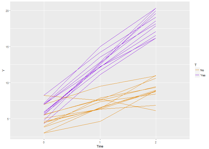Again, we recover the true parameters. And this time, if we look at the estimated correlation, we see that indeed the outcomes are correlated within each individual. The estimate is 0.71, very close to the the “true” value 0.7.

fit <- geeglm(Y ~ factor(T) + period + factor(T) * period, family = gaussian(link = "identity"), 
    data = longData, id = id, corstr = "exchangeable")

summary(fit)

## 
## Call:
## geeglm(formula = Y ~ factor(T) + period + factor(T) * period, 
##     family = gaussian(link = "identity"), data = longData, id = id, 
##     corstr = "exchangeable")
## 
##  Coefficients:
##                     Estimate Std.err Wald Pr(>|W|)    
## (Intercept)           5.0636  0.0762 4411   <2e-16 ***
## factor(T)Yes          1.4945  0.1077  192   <2e-16 ***
## period                2.4972  0.0303 6798   <2e-16 ***
## factor(T)Yes:period   3.5204  0.0426 6831   <2e-16 ***
## ---
## Signif. codes:  0 '***' 0.001 '**' 0.01 '*' 0.05 '.' 0.1 ' ' 1
## 
## Estimated Scale Parameters:
##             Estimate Std.err
## (Intercept)     3.07   0.117
## 
## Correlation: Structure = exchangeable  Link = identity 
## 
## Estimated Correlation Parameters:
##       Estimate Std.err
## alpha    0.711  0.0134
## Number of clusters:   1000   Maximum cluster size: 3

Another way to generate correlated data

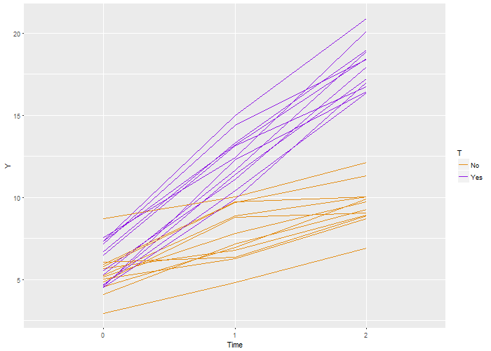
A second way to generate correlated data is through an individual level random-effect or random intercept. This could be considered some unmeasured characteristic of the individuals (which happens to have a convenient normal distribution with mean zero). This random effect contributes equally to all instances of an individuals outcomes, but the outcomes for a particular individual deviate slightly from the hypothetical straight line as a result of unmeasured noise.

ydef1 <- defData(varname = "randomEffect", dist = "normal", formula = 0, variance = sqrt(3))
ydef2 <- defDataAdd(varname = "Y", dist = "normal", formula = "5 + 2.5*period + 1.5*T + 3.5*period*T + randomEffect", 
    variance = 1)

indData <- genData(24, ydef1)
indData <- trtAssign(indData, nTrt = 2, balanced = TRUE, grpName = "T")

indData[1:6]

##    id T randomEffect
## 1:  1 0      -1.3101
## 2:  2 1       0.3423
## 3:  3 0       0.5716
## 4:  4 1       2.6723
## 5:  5 0      -0.9996
## 6:  6 1      -0.0722

longData <- addPeriods(indData, nPeriods = 3, idvars = "id")
longData <- addColumns(dtDefs = ydef2, longData)

longData[, `:=`(T, factor(T, labels = c("No", "Yes")))]

ggplot(data = longData, aes(x = factor(period), y = Y)) + geom_line(aes(color = T, 
    group = id)) + scale_color_manual(values = c("#e38e17", "#8e17e3")) + xlab("Time")

fit <- geeglm(Y ~ factor(T) + period + factor(T) * period, family = gaussian(link = "identity"), 
    data = longData, id = id, corstr = "exchangeable")
summary(fit)

## 
## Call:
## geeglm(formula = Y ~ factor(T) + period + factor(T) * period, 
##     family = gaussian(link = "identity"), data = longData, id = id, 
##     corstr = "exchangeable")
## 
##  Coefficients:
##                     Estimate Std.err Wald Pr(>|W|)    
## (Intercept)           4.9230  0.0694 5028   <2e-16 ***
## factor(T)Yes          1.4848  0.1003  219   <2e-16 ***
## period                2.5310  0.0307 6793   <2e-16 ***
## factor(T)Yes:period   3.5076  0.0449 6104   <2e-16 ***
## ---
## Signif. codes:  0 '***' 0.001 '**' 0.01 '*' 0.05 '.' 0.1 ' ' 1
## 
## Estimated Scale Parameters:
##             Estimate Std.err
## (Intercept)     2.63  0.0848
## 
## Correlation: Structure = exchangeable  Link = identity 
## 
## Estimated Correlation Parameters:
##       Estimate Std.err
## alpha    0.619  0.0146
## Number of clusters:   1000   Maximum cluster size: 3

I sent all this back to my correspondent, but I haven’t heard yet if either of these solutions meets her needs. I certainly hope so. Speaking of which, if there are specific topics you’d like me to discuss related to simstudy, definitely get in touch, and I will try to write something up.