The Herfindahl-Hirschman Index (HHI) is a widely used measure of concentration in a variety of fields including, business, economics, political science, finance, and many others. Though simple to calculate (summed squared market shares of firms/actors in a single market/space), calculation of the HHI can get onerous, especially as the number of firms/actors increases and the time period grows. Thus, I decided to write a package aimed at streamlining and simplifying calculation of HHI scores. The package, hhi, calculates the concentration of a market/space based on a supplied vector of values corresponding with shares of all individual firms/actors acting in that space. The package is available on CRAN.
# First, install the "hhi" package, then load the library
install.packages("hhi")
library(hhi)

# Next, read in data: US Men's Footwear Company Market Shares, 2012-2017
footwear = read.table(".../footwear.txt")

# Now, call the "hhi" command to calculate HHI for 2017
hhi(footwear, "ms.2017") # first the df, then the shares variable in quotes
Often, the HHI is used as a measure of competition, with 10,000 equaling perfect monopoly (100^2) and 0.0 equaling perfect competition. As such, we can see that the U.S. men’s footwear industry in 2017 seems relatively competitive. Yet, to say anything substantive about the men’s U.S. footwear market, we really need a comparison of HHI scores for this market over time. This is where the second command comes in.
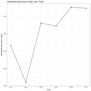
Let’s return to our men’s U.S. footwear example to see how the function works in practice. First, we need to calculate the HHI scores for each year in the data file (2012-2017), and store those as objects to make a data frame of HHI scores corresponding to individual years. Then, we simply call the plot_hhi command and generate a simple, pleasing plot of HHI scores over time. This will give us a much better sense of how our 2017 HHI score above compares with other years in this market. See the code below, followed by the output.
# First, calculate and store HHI for each year in the data file (2012-2017)
hhi.12 = hhi(footwear, "ms.2012")
hhi.13 = hhi(footwear, "ms.2013")
hhi.14 = hhi(footwear, "ms.2014")
hhi.15 = hhi(footwear, "ms.2015")
hhi.16 = hhi(footwear, "ms.2016")
hhi.17 = hhi(footwear, "ms.2017")

# Combine and create df for plotting
hhi = rbind(hhi.12, hhi.13, hhi.14, hhi.15, hhi.16, hhi.17)

year = c(2012, 2013, 2014, 2015, 2016, 2017)

hhi.data = data.frame(year, hhi)

# Finally, generate HHI time series plot using the "plot_hhi" command
plot_hhi(hhi.data, "year", "hhi")
These lines of code will give us the following plot of HHI scores for each year in the data set.

Interestingly, the men’s U.S. footwear industry seems to be getting slightly less competitive (higher HHI scores) from 2012 to 2017, on average. To say anything substantive about this trend, though, would obviously require more sophisticated methods as well as a longer time series. Yet, the value of the hhi package is allowing for quick calculation and visualization of HHI scores over time. You can download the package from CRAN or directly from the package installation context in RStudio. And as always, if you have any questions or find any bugs requiring fixing, please feel free to contact me.
Herfindahl, Orris C. 1950. “Concentration in the steel industry.” Ph.D. dissertation, Columbia University.
Hirschman, Albert O. 1945. “National power and structure of foreign trade.” Berkeley, CA: University of California Press.
Rhoades, Stephen A. 1993. “The herfindahl-hirschman index.” Federal Reserve Bulletin 79: 188.