Trend Forecasting Models and Seasonality with Time Series

Interested in publishing a one-time post on R-bloggers.com? Press here to learn how.

---

Gasoline prices always is an issue in Turkey; because Turkish people love to drive where they would go but they complain about the prices anyway. I wanted to start digging for the last seven years’ prices and how they went. I have used unleaded gasoline 95 octane prices from Petrol Ofisi which is a fuel distribution company in Turkey. I arranged the prices monthly between 2013 and 2020 as the Turkish currency, Lira (TL). The dataset is here

head(gasoline_df)
#        date gasoline
#1 2013-01-01     4.67
#2 2013-02-01     4.85
#3 2013-03-01     4.75
#4 2013-04-01     4.61
#5 2013-05-01     4.64
#6 2013-06-01     4.72

First of all, I wanted to see how gasoline prices went during the period and analyze the fitted trend lines.

#Trend lines 
library(tidyverse)

ggplot(gasoline_df, aes(x = date, y = gasoline)) + geom_point() +
  stat_smooth(method = 'lm', aes(colour = 'linear'), se = FALSE) +
  stat_smooth(method = 'lm', formula = y ~ poly(x,2), aes(colour = 'quadratic'), se= FALSE) +
  stat_smooth(method = 'lm', formula = y ~ poly(x,3), aes(colour = 'cubic'), se = FALSE)+
  stat_smooth(data=exp.model.df, method = 'loess',aes(x,y,colour = 'exponential'), se = FALSE) 

Because the response variable is measured by logarithmic in the exponential model, we have to get the exponent of it and create a different data frame for the exponential trend line.

#exponential trend model
exp.model <- lm(log(gasoline)~date,data = gasoline_df) 
exp.model.df <- data.frame(x=gasoline_df$date,
                           y=exp(fitted(exp.model)))

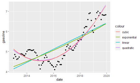
As we see above, the cubic and quadratic models almost overlap each other and they seem to be fit better to the data. However, we will analyze each model in detail.

The Forecasting Trend Models

The linear trend; $latex y_{t}&s=1$, the value of the series at given time, $latex t&s=1$, is described as:

$latex y_{t}&s=1=\beta_{0}+\beta_{1}t&s=1+\epsilon_{t}$

$latex \beta_{0}&s=1$ and $latex \beta_{1}&s=1$ are the coefficients.

model_linear <- lm(data = gasoline_df,gasoline~date)

Above, we created a model variable for the linear trend model. In order to compare the models, we have to extract the adjusted coefficients of determination, that is used to compare regression models with a different number of explanatory variables, from each trend models.

Adjusted $latex R^2&s=1=1-(1-R^2&s=1)(\frac {n-1} {n-k-1})$
$latex n$: sample size
$latex k$: number of variables
$latex R^2&s=1$: coefficient of determination which is the square of correlation of observation values with predicted values: $latex r^2_{y \hat {y}}$

adj_r_squared_linear <- summary(model_linear) %>% 
  .$adj.r.squared %>% 
  round(4)

The exponential trend; unlike the linear trend, allows the series to increase at an increasing rate in each period, is described as:
$latex \ln(y_{t}&s=1)=\beta_{0}+\beta_{1}t&s=1+\epsilon_{t}$. $latex \ln(y_{t}&s=1)$ is a natural logarithm of the response variable.

To make predictions on the fitted model, we use exponential function as  $latex \hat{y_{t}}&s=1=exp(b_{0}+b_{1}t+s_{e}^2/2)$ because the dependent variable was transformed by a natural logarithmic function. In order for $latex \hat{y_{t}}&s=1$ not to be under the expected value of $latex y{t}&s=1$, we add half of the residual standard error's square. In order to find $latex s_{e}&s=2$, we execute the summary function as below. In addition, we can see the level of significance of the coefficients and the model. As we see below, because the p-value of the coefficients and the model are less than 0.05, they are significant at the %5 level of significance.

summary(model_exponential)

#Call:
#lm(formula = log(gasoline) ~ date, data = gasoline_df)

#Residuals:
#      Min        1Q    Median        3Q       Max 
#-0.216180 -0.083077  0.009544  0.087953  0.151469 

#Coefficients:
#              Estimate Std. Error t value Pr(<|t|)    
#(Intercept) -1.0758581  0.2495848  -4.311  4.5e-05 ***
#date         0.0001606  0.0000147  10.928  < 2e-16 ***
#---
#Signif. codes:  0 ‘***’ 0.001 ‘**’ 0.01 ‘*’ 0.05 ‘.’ 0.1 ‘ ’ 1

#Residual standard error: 0.09939 on 82 degrees of freedom
#Multiple R-squared:  0.5929,  Adjusted R-squared:  0.5879 
#F-statistic: 119.4 on 1 and 82 DF,  p-value: < 2.2e-16

We create an exponential model variable.

model_exponential <- lm(data = gasoline_df,log(gasoline)~date)

To get adjusted $latex R^2&s=1$, we first transform the predicted variable.

library(purrr)

y_predicted <- model_exponential$fitted.values %>% 
  map_dbl(~exp(.+0.09939^2/2))

And then, we execute the formula shown above to get adjusted $latex R^2&s=1$

r_squared_exponential <- (cor(y_predicted,gasoline_df$gasoline))^2

adj_r_squared_exponential <- 1-(1-r_squared_exponential)*
  ((nrow(gasoline_df)-1)/(nrow(gasoline_df)-1-1))

Sometimes a time-series changes the direction with respect to many reasons. This kind of target variable is fitted to polynomial trend models. If there is one change of direction we use the quadratic trend model.

$latex y_{t}&s=1=\beta_{0}+\beta_{1}t+\beta_{2}t^2+\epsilon$

If there are two change of direction we use the cubic trend models:

$latex y_{t}&s=1=\beta_{0}+\beta_{1}t+\beta_{2}t^2+\beta_{3}t^3+\epsilon$

Then again, we execute the same process as we did in the linear model.

#Model variables
model_quadratic <- lm(data = df,gasoline~poly(date,2))
model_cubic <- lm(data = df,gasoline~poly(date,3))

#adjusted coefficients of determination
adj_r_squared_quadratic <- summary(model_quadratic) %>% 
  .$adj.r.squared

adj_r_squared_cubic <- summary(model_cubic) %>% 
  .$adj.r.squared

In order to compare all models, we create a variable that gathers all adjusted $latex R^2&s=1$.

adj_r_squared_all <- c(linear=round(adj_r_squred_linear,4),
                   exponential=round(adj_r_squared_exponential,4),
                   quadratic=round(adj_r_squared_quadratic,4),
                   cubic=round(adj_r_squared_cubic,4))

As we can see below, the results justify the graphic we built before; polynomial models are much better than the linear and exponential models. Despite polynomial models look almost the same, the quadratic model is slightly better than the cubic model.

adj_r_squared_all
     #linear exponential   quadratic       cubic 
     #0.6064      0.6477      0.8660      0.8653

Seasonality

The seasonality component represents the repeats in a specific period of time. Time series with weekly monthly or quarterly observations tend to show seasonal variations that repeat every year. For example, the sale of retail goods increases every year in the Christmas period or the holiday tours increase in the summer. In order to detect seasonality, we use decomposition analysis.

Decomposition analysis: $latex T, S, I&s=1$, are trend, seasonality and random components of the series respectively. When seasonal variation increases as the time series increase, we'd use the multiplicative model.

$latex y_{t}&s=1=T_{t} \times S_{t} \times I_{t}$

If the variation looks constant, we should use additive model. 

$latex y_{t}&s=1=T_{t} + S_{t} + I_{t}$

To find which model is fit, we have to look at it on the graph.

#we create a time series variable for the plot
gasoline_ts <- ts(gasoline_df$gasoline,start = c(2013,1),end = c(2019,12),frequency = 12)
#The plot have all the components of the series(T, S, I)
plot(gasoline_ts,lwd=2,ylab="Gasoline")

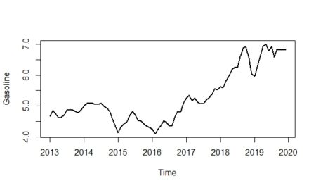
As we can see from the plot above, it seems that the multiplicative model would be more fit for the data; especially if we look at between 2016-2019. When we analyze the graph, we see some conjuncture variations caused by the expansion or contraction of the economy. Unlike seasonality, conjuncture fluctuations can be several months or years in length.

Additionally, the magnitude of conjuncture fluctuation can change in time because the fluctuations differ in magnitude and length so they are hard to reflect with historical data; because of that, we neglected the conjuncture component of the series.

Extracting the seasonality

Moving averages (ma) usually be used to separate the effect of a trend from seasonality.

$latex m\,\,term\,\,moving\,\,averages&s=1=\frac {Average\,\,of\,\,the\,\,last\,\,m\,\,observations} {m}$

We use the cumulative moving average (CMA), which is the average of two consecutive averages, to show the even-order moving average. For example; first two ma terms are $latex \bar{y}_{6.5}&s=1$ and $latex \bar{y}_{7.5}&s=1$ but there are no such terms in the original series; therefore we average the two terms to find CMA term matched up in the series:

 $latex \bar y_7&s=3=$$latex \frac {\bar y_{6,5}&s=3+\bar y_{7,5}} {2}$

The default value of the 'centre' argument of the ma function remains TRUE to get CMA value. 

library(forecast)

gasoline_trend <- forecast::ma(gasoline_ts,12)

If noticed, $latex \bar y_{t}&s=1$ eliminates both seasonal and random variations; hence: $latex \bar y_{t}&s=1=T_{t}$

Since $latex y_{t}&s=1=T_{t} \times S_{t} \times I_{t}$ and $latex \bar y_{t}&s=1=T_{t}$, the detrend variable is found by: $latex \frac {\bar y_{t}} {y_{t}}&s=1=S_{t} \times I_{t}$; it is also called ratio-to moving averages method.

gasoline_detrend <- gasoline_ts/gasoline_trend

Each month has multiple ratios, where each ratio coincides with a different year; in this sample, each month has seven different ratios. The arithmetic average is used to determine common value for each month; by doing this, we eliminate the random component and subtract the seasonality from the detrend variable. It is called the unadjusted seasonal index.

unadjusted_seasonality <- sapply(1:12, function(x) mean(window(gasoline_detrend,c(2013,x),c(2019,12),deltat=1),na.rm = TRUE)) %>% round(4)

Seasonal indexes for monthly data should be completed to 12, with an average of 1; in order to do that each unadjusted seasonal index is multiplied by 12 and divided by the sum of 12 unadjusted seasonal indexes.

adjusted_seasonality <- (unadjusted_seasonality*(12/sum(unadjusted_seasonality))) %>% 
                        round(4)

The average of all adjusted seasonal indices is 1; if an index is equal to 1, that means there would be no seasonality. In order to plot seasonality:

#building a data frame to plot in ggplot
adjusted_seasonality_df <- data_frame(
  months=month.abb,
  index=adjusted_seasonality)

#converting char month names to factor sequentially
adjusted_seasonality_df$months <- factor(adjusted_seasonality_df$months,levels = month.abb)


ggplot(data = adjusted_seasonality_df,mapping = aes(x=months,y=index))+
 geom_point(aes(colour=months))+
 geom_hline(yintercept=1,linetype="dashed")+
 theme(legend.position = "none")+
 ggtitle("Seasonality of Unleaded Gasoline Prices for 95 Octane")+
 theme(plot.title = element_text(h=0.5))

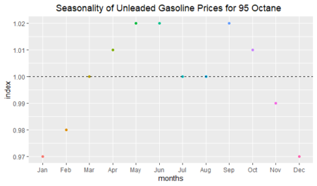
As we can see above, there is approximately a three-percent seasonal decrease in January and December; on the other hand, there is a two-percent seasonal increase in May and June. Seasonality is not seen in March, July, and August; because their index values are approximately equal to 1.

Decomposing the time series graphically

We will first show the trend line on the time series.

#Trend is shown by red line
plot(gasoline_ts,lwd=2,ylab="Gasoline")+
lines(gasoline_trend,col="red",lwd=3)

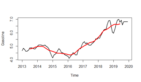
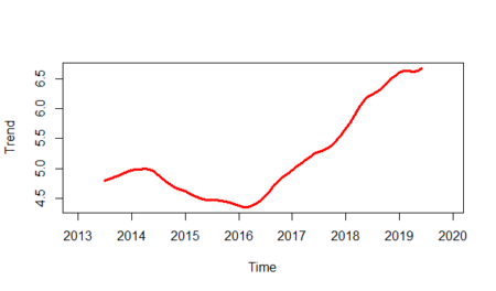
And will isolate the trend line from the plot:

plot(gasoline_trend,lwd=3,col="red",ylab="Trend")

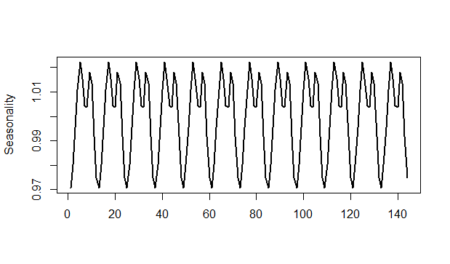
Let's see the seasonality line:

plot(as.ts(rep(unadjusted_seasonality,12)),lwd=2,ylab="Seasonality",xlab="")

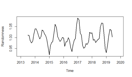
And finally, we will show the randomness line; in order to do that:
$latex I_{t}&s=1=\frac {y_{t}} {S_{t}\times T_{t}}$

randomness <- gasoline_ts/(gasoline_trend*unadjusted_seasonality)
plot(randomness,ylab="Randomness",lwd=2)

References

Sanjiv Jaggia, Alison Kelly (2013). Business Intelligence: Communicating with Numbers.