Introducing latent2likert v1.2.1: Converting Latent Variables into Likert Scale Responses

Introduction Package logo


In social sciences, variables of interest are often conceptualized as latent variables—hidden continuous variables measured through Likert scale questions, typically categorized as Strongly disagree, Disagree, Neutral, Agree, and Strongly agree. Researchers frequently aim to uncover these latent variables using various statistical techniques.

Accurate modeling of survey data is crucial for comparative analysis through simulation, especially when applying statistical techniques that require metric data. The latent2likert package addresses this need by providing an effective algorithm to simulate Likert response variables from hypothetical latent variables. This post introduces the features of the latent2likert package.

Simulating Likert Scale Responses

Using the rlikert function, you can generate random responses to Likert scale questions based on specified means and standard deviations of latent variables, with optional settings for skewness and correlations.

Reproducing Rating-Scale Data

From existing survey data, you can estimate the values of latent parameters using the estimate_params function. You can then generate new responses using the estimated parameters to create a new dataset with very similar properties.

Further Reading

For more detailed information and practical examples, please refer to the package website and vignette. The implemented algorithms are described in the function reference.

Related R Packages

To simulate Likert scale responses, the draw_likert function from the fabricatr package can recode a latent variable into a Likert response variable by specifying intervals that subdivide the continuous range. However, the latent2likert package offers an advantage by automatically calculating optimal intervals that minimize distortion between the latent variable and the Likert response variable for both normal and skew normal latent distributions, eliminating the need to manually specify the intervals.

There are also alternative approaches that do not rely on latent distributions. One method involves directly defining a discrete probability distribution and sampling from it using the sample function in R or the likert function from the wakefield package. Another approach is to specify the means, standard deviations, and correlations among Likert response variables. For this, you can use LikertMakeR or SimCorMultRes to generate correlated multinomial responses.

Additionally, you can define a data-generating process. For those familiar with item response theory, the mirt package allows users to specify discrimination and difficulty parameters for each response category.
“Those who can, do;  those who can’t – use computer simulation.”

     “Those who can, do;  those who can’t – use computer simulation.”  This quote was inspired by playwright George Bernard Shaw.  Computer simulation is a powerful tool that attempts to reproduce the behavior of some real-world system by sampling from one or more probability distributions.  It can help explain and illustrate difficult concepts such as the Monty Hall game show problem.  It can also solve problems that are hard or impossible to solve directly. 

     One example of a problem of this latter type is the probability distribution of the sum of n independent random variables each having probability distribution g, where n is also a random variable having probability distribution f.  This is a special case of a statistical subject called convolutions, where one calculates the convolution of all possible values of the individual distributions.  For certain choices of f and g, such as Poisson for f and gamma for g, the resulting convolution is an integrateable function and there is no need for simulation.  But for many choices of f and g, simulation or some other numerical method is needed.
     A real-world use of this type of simulation is in modeling loss events of a business entity such as a bank or insurance company.  The entity will have some random number of events n per year of random sizes that is modeled by a frequency distribution f such as Poisson or negative binomial.  A number n is randomly selected from the frequency distribution.  Then n random numbers are randomly selected from a severity distribution g such as lognormal or gamma to simulate the sizes of the n loss events.  The n loss amounts are added to produce a total value of losses for one year.  The process is repeated some large number of times, say 10,000, and the 10,000 numbers are ranked.  If the entity is interested in the 99.9th percentile such loss, that value is the 9,990th largest value.
     Base R provides functions to simulate from many probability distributions.  For example, rpois(n, lamda) produces n Poisson distributed samples from a distribution having population mean lambda.  Poisson is a single parameter distribution with variance equal to the mean.  An alternative frequency distribution with a more flexible option for the variance is the negative binomial distribution.  Its R function is rnbinom(n, mu, size) which produces n negative binomial distributed samples from a distribution having population mean mu and dispersion parameter size, where size = mu^2 / (variance – mu).
     Most severity distributions are not symmetrical but rather are positively skewed with low mean and long positive tail.  A random variable is lognormally distributed if the logarithm of the random variable  is normally distributed.  Its R function is rlnorm(n, meanlog, sdlog) which produces n lognormally distributed samples from a distribution having population mean m and standard deviation s, and here meanlog = LN(m) – .5*LN((s/m)^2 + 1)) and sdlog = .5*LN((s/m)^2+1)).
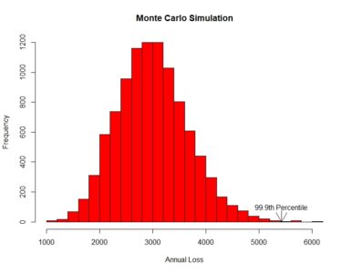
     It is helpful to plot the resulting histogram of the 10,000 simulations.  The real-world purpose of the exercise may be to identify the 99.9th percentile value.    The R quantile function quantile(x, probs) returns the percentile value equal to probs.  To display the percentile value on a plot, use the text and arrow functions.  R has a text function that adds text a plot, text(x, y, label), which adds a label at coordinate (x,y).  Further, R has an arrows function, arrows(x0, y0, x1, y1, code=2), which draws an arrow from (x0, y0) to (x1, y1)  with code 2 drawing the arrowhead at (x1, y1).
     The following is the R code and resulting histogram plot of a negative binomial frequency and lognormal severity simulation.  The user input values are based on the mean and standard deviation values of a dataset.

# Monte Carlo simulation. Negative binomial frequency, lognormal severity. 

# negbinom
nb_m <- 50 # This is a user input.
nb_sd <- 10 # This is a user input.
nb_var <- nb_sd^2
nb_size <- nb_m^2/(nb_var – nb_m)

# lognorm
xbar <- 60 # This is a user input.
sd <- 40 # This is a user input.
l_mean <- log(xbar) – .5*log((sd/xbar)^2 + 1)
l_sd <- sqrt(log((sd/xbar)^2 + 1))

num_sims <- 10000 # This is a user input.
set.seed(1234) # This is a user input.
rtotal <- vector()

for (i in 1:num_sims)
{
nb_random <- rnbinom(n=1, mu=nb_m, size=nb_size)
l_random <- rlnorm(nb_random, meanlog=l_mean, sdlog=l_sd)
rtotal[i] <- sum(l_random)
}

rtotal <- sort(rtotal)
m <- round(mean(rtotal), digits=0)
percentile_999 <- round(quantile(rtotal, probs=.999), digits=0)

print(paste(“Mean = “, m, ” 99.9th percentile = “, percentile_999))

hist(rtotal, breaks=20, col=”red”, xlab=”Annual Loss”, ylab=”Frequency”,
main=”Monte Carlo Simulation”)
text(percentile_999, 100, “99.9th Percentile”)
arrows(percentile_999,75, percentile_999,0, code=2)

[contact-form][contact-field label=”Name” type=”name” required=”true” /][contact-field label=”Email” type=”email” required=”true” /][contact-field label=”Website” type=”url” /][contact-field label=”Message” type=”textarea” /][/contact-form]