Imagine you need to find the average height of 20-year olds. One way is to go around and measure each person individually. But that seems quite a bit of work, doesn’t it? Luckily, there’s a better way. Inferential statistics allows us to use samples to draw conclusions about the population. In other words, we can get a small group of people and use their characteristics to estimate the characteristics of the entire group.
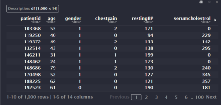
To see how this works in practice, let’s take a look at a dataset from Kaggle. This platform provides a wealth of data sets from various fields, each offering unique challenges for R users. Here, we’ll be using a dataset on Cardiovascular diseases compiled by Jocelyn Dumlao.
This dataset originates from a renowned multispecialty hospital situated in India, encompassing a comprehensive array of health-related information. Comprising an extensive structure of 1000 columns and 14 rows, this dataset plays a pivotal role in the early detection of diseases.
Let us see how to import this into RStudio. The dataset is imported into RStudio using the library ‘readr’ (this is only if the dataset is in .csv format). Replace “File path” with the path of your downloaded dataset.
library(readr)
cardio <- read.csv("File path")
Just type in the name of the variable you used to import the dataset so that you can view the entire dataset in RStudio.
cardio

The first 6 rows of the dataset can be viewed using the ‘head’ function.
top_6=head(cardio)
top_6
Similarly, the last 6 rows of the dataset can be viewed using the ‘tail’ function.
bottom_6=tail(cardio)
bottom_6
The dimension of the dataset (number of rows and columns) can be found out using the ‘dim’ function.
dimension=dim(cardio)
dimension
The entire dataset can be termed as population and all the population parameters can be easily found. The mean of a target variable in the population is calculated by the ‘mean’ function. Below, we choose serumcholestrol as the target variable.
mean_chol=mean(cardio$serumcholestrol)
mean_chol
So, we can infer that the average serumcholestrol levels in the patient population taken from the hospital is 311.447.
There also exists a function to calculate the standard deviation of a dataset.
std_chol=sd(cardio$serumcholestrol)
std_chol
From this value, it can be understood that the values of serumcholestrol lies 132.4438 below or above the mean level.
We take a random sample of size 100 where our target variable is serumcholestrol. If you want to take a random sample with replacement, give the third argument as TRUE. Here, we’re taking a sample without replacement.
sample_1=sample(cardio$serumcholestrol,100,FALSE)
sample_1
mean_sample_chol=mean(sample_1)
mean_sample_chol
The mean of the sample that we selected is 317.51. This mean can be used to calculate the test statistic which further can be used to make decisions about the null hypothesis(whether to accept or reject).
Calculating the standard error of the sample


Getting the standard deviation of a dataset gives us many insights. Standard deviation provides the spread of the data around the mean. The standard deviation of sampling distribution is called standard error.
std_error=sd(sample_1)
std_error
Plotting the sample distribution in histogram with x-axis as frequency and y-axis as Cholesterol levels.To get a sampling distribution, we repeatedly take samples 1000 times. This is done using the replicate function, which repeatedly evaluates an expression a given number of times.
samp_dist_1=replicate(1000,mean(sample(cardio$serumcholestrol,100,replace=TRUE)))
samp_dist_1
variance_sample_1=var(samp_dist_1)
variance_sample_1
Now let us see how increasing the sample size affects the variance of the sample.
Increasing the sample size by 200
sample_2=sample(cardio$serumcholestrol,200,FALSE)
sample_2
mean_sample_chol=mean(sample_2)
mean_sample_chol
Calculating the standard error of the sample2
std_error=sd(sample_2)
std_error
The standard error of sample2 is 135.9615 .

We repeat the previous steps to obtain a sampling distribution.
samp_dist_2=replicate(1000,mean(sample(cardio$serumcholestrol,200,replace=TRUE)))
samp_dist_2
hist(samp_dist_2,main="Sampling distribution of serum_cholestrol",xlab = "Frequency",ylab = "Cholestrol Levels", col = "skyblue")
variance_sample_2=var(samp_dist_2)
variance_sample_2
Authors: Aadith Joseph Mathew, Amrutha Paalathara, Devika S Vinod, Jyosna Philip