How to Perform Hierarchical Clustering using R

Interested in publishing a one-time post on R-bloggers.com? Press here to learn how.

---

What is Hierarchical Clustering?

Clustering is a technique to club similar data points into one group and separate out dissimilar observations into different groups or clusters. In Hierarchical Clustering, clusters are created such that they have a predetermined ordering i.e. a hierarchy. For example, consider the concept hierarchy of a library. A library has many sections, each section would have many books, and the books would be grouped according to their subject, let’s say. This forms a hierarchy. In Hierarchical Clustering, this hierarchy of clusters can either be created from top to bottom, or vice-versa. Hence, it’s two types namely – Divisive and Agglomerative. Let’s discuss it in detail.

Divisive Method

In Divisive method we assume that all of the observations belong to a single cluster and then divide the cluster into two least similar clusters. This is repeated recursively on each cluster until there is one cluster for each observation. This technique is also called DIANA, which is an acronym for Divisive Analysis.

Agglomerative Method

It’s also known as Hierarchical Agglomerative Clustering (HAC) or AGNES (acronym for Agglomerative Nesting). In this method, each observation is assigned to its own cluster. Then, the similarity (or distance) between each of the clusters is computed and the two most similar clusters are merged into one. Finally, steps 2 and 3 are repeated until there is only one cluster left.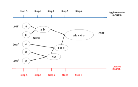


Please note that Divisive method is good for identifying large clusters while Agglomerative method is good for identifying small clusters. We will proceed with Agglomerative Clustering for the rest of the article. Since, HAC’s account for the majority of hierarchical clustering algorithms while Divisive methods are rarely used. I think now we have a general overview of Hierarchical Clustering. Let’s also get ourselves familiarized with the algorithm for it.

HAC Algorithm

Given a set of N items to be clustered, and an NxN distance (or similarity) matrix, the basic process of Johnson’s (1967) hierarchical clustering is –

1. Assign each item to its own cluster, so that if you have N items, you now have N clusters, each containing just one item. Let the distances (similarities) between the clusters equal the distances (similarities) between the items they contain.
2. Find the closest (most similar) pair of clusters and merge them into a single cluster, so that now you have one less cluster.
3. Compute distances (similarities) between the new cluster and each of the old clusters.
4. Repeat steps 2 and 3 until all items are clustered into a single cluster of size N.

In Steps 2 and 3 here, the algorithm talks about finding similarity among clusters. So, before any clustering is performed, it is required to determine the distance matrix that specifies the distance between each data point using some distance function (Euclidean, Manhattan, Minkowski, etc.). Then, the matrix is updated to specify the distance between different clusters that are formed as a result of merging. But, how do we measure the distance (or similarity) between two clusters of observations? For this, we have three different methods as described below. These methods differ in how the distance between each cluster is measured.

Single Linkage

It is also known as the connectedness or minimum method. Here, the distance between one cluster and another cluster is taken to be equal to the shortest distance from any data point of one cluster to any data point in another. That is, distance will be based on similarity of the closest pair of data points as shown in the figure. It tends to produce long, “loose” clusters. Disadvantage of this method is that it can cause premature merging of groups with close pairs, even if those groups are quite dissimilar overall.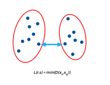 

Complete Linkage

This method is also called the diameter or maximum method. In this method, we consider similarity of the furthest pair. That is, the distance between one cluster and another cluster is taken to be equal to the longest distance from any member of one cluster to any member of the other cluster. It tends to produce more compact clusters. One drawback of this method is that outliers can cause close groups to be merged later than what is optimal.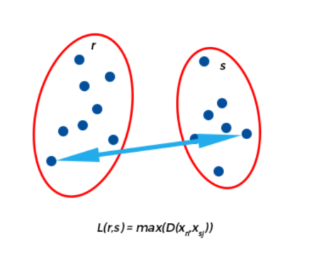 

Average Linkage

In Average linkage method, we take the distance between one cluster and another cluster to be equal to the average distance from any member of one cluster to any member of the other cluster. A variation on average-link clustering is the UCLUS method of D’Andrade (1978) which uses the median distance instead of mean distance.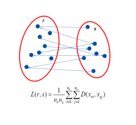 

Ward’s Method

Ward’s method aims to minimize the total within-cluster variance. At each step the pair of clusters with minimum between-cluster distance are merged. In other words, it forms clusters in a manner that minimizes the loss associated with each cluster. At each step, the union of every possible cluster pair is considered and the two clusters whose merger results in minimum increase in information loss are combined. Here, information loss is defined by Ward in terms of an error sum-of-squares criterion (ESS). If you want a mathematical treatment of this visit this link.

The following table describes the mathematical equations for each of the methods —


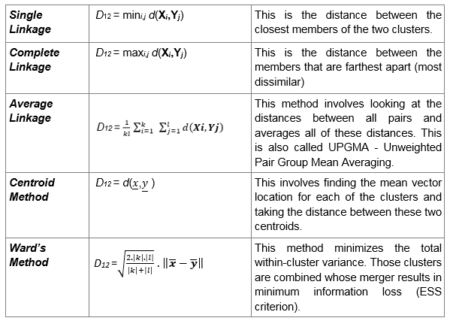
Where,

• X1, X2, , Xk = Observations from cluster 1
• Y1, Y2, , Yl = Observations from cluster 2
• d (x, y) = Distance between a subject with observation vector x and a subject with observation vector y
• ||.|| = Euclidean norm

Implementing Hierarchical Clustering in R

Data Preparation

To perform clustering in R, the data should be prepared as per the following guidelines –

1. Rows should contain observations (or data points) and columns should be variables.
2. Check if your data has any missing values, if yes, remove or impute them.
3. Data across columns must be standardized or scaled, to make the variables comparable.

We’ll use a data set called ‘Freedman’ from the ‘car’ package. The ‘Freedman’ data frame has 110 rows and 4 columns. The observations are U. S. metropolitan areas with 1968 populations of 250,000 or more. There are some missing data. (Make sure you install the car package before proceeding)

data <- car::Freedman

To remove any missing value that might be present in the data, type this:
data <- na.omit(data)

This simply removes any row that contains missing values. You can use more sophisticated methods for imputing missing values. However, we’ll skip this as it is beyond the scope of the article. Also, we will be using numeric variables here for the sake of simply demonstrating how clustering is done in R. Categorical variables, on the other hand, would require special treatment, which is also not within the scope of this article. Therefore, we have selected a data set with numeric variables alone for conciseness.

Next, we have to scale all the numeric variables. Scaling means each variable will now have mean zero and standard deviation one. Ideally, you want a unit in each coordinate to represent the same degree of difference. Scaling makes the standard deviation the unit of measurement in each coordinate. This is done to avoid the clustering algorithm to depend to an arbitrary variable unit. You can scale/standardize the data using the R function scale:

data <- scale(data)

Implementing Hierarchical Clustering in R

There are several functions available in R for hierarchical clustering. Here are some commonly used ones:

• ‘hclust’ (stats package) and ‘agnes’ (cluster package) for agglomerative hierarchical clustering
• ‘diana’ (cluster package) for divisive hierarchical clustering

Agglomerative Hierarchical Clustering

For ‘hclust’ function, we require the distance values which can be computed in R by using the ‘dist’ function. Default measure for dist function is ‘Euclidean’, however you can change it with the method argument. With this, we also need to specify the linkage method we want to use (i.e. “complete”, “average”, “single”, “ward.D”).

# Dissimilarity matrix
d <- dist(data, method = "euclidean")
# Hierarchical clustering using Complete Linkage
hc1 <- hclust(d, method = "complete" )
# Plot the obtained dendrogram
plot(hc1, cex = 0.6, hang = -1)

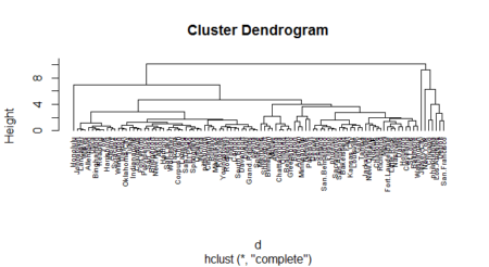
Another alternative is the agnes function. Both of these functions are quite similar; however, with the agnes function you can also get the agglomerative coefficient, which measures the amount of clustering structure found (values closer to 1 suggest strong clustering structure).

# Compute with agnes (make sure you have the package cluster)
hc2 <- agnes(data, method = "complete")

# Agglomerative coefficient
hc2$ac

## [1] 0.9317012
Let’s compare the methods discussed

# vector of methods to compare
m <- c( "average", "single", "complete", "ward")
names(m) <- c( "average", "single", "complete", "ward")

# function to compute coefficient
ac <- function(x) {
  agnes(data, method = x)$ac
}
map_dbl(m, ac)      

## from ‘purrr’ package
## average single complete ward

## 0.9241325 0.9215283 0.9317012 0.9493598

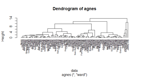
Ward’s method gets us the highest agglomerative coefficient. Let us look at its dendogram.
hc3 <- agnes(data, method = "ward")
pltree(hc3, cex = 0.6, hang = -1, main = "Dendrogram of agnes")

Divisive Hierarchical Clustering

The function ‘diana’ in the cluster package helps us perform divisive hierarchical clustering. ‘diana’ works similar to ‘agnes’. However, there is no method argument here, and, instead of agglomerative coefficient, we have divisive coefficient.

# compute divisive hierarchical clustering
hc4 <- diana(data)

# Divise coefficient
hc4$dc

## [1] 0.9305939

# plot dendrogram
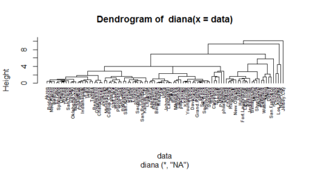
pltree(hc4, cex = 0.6, hang = -1, main = "Dendrogram of diana")

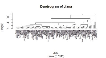
A dendogram is a cluster tree where each group is linked to two or more successor groups. These groups are nested and organized as a tree. You could manage dendograms and do much more with them using the package “dendextend”. Check out the vignette of the package here:
https://cran.r-project.org/web/packages/dendextend/vignettes/Quick_Introduction.html

Great! So now we understand how to perform clustering and come up with dendograms. Let us move to the final step of assigning clusters to the data points. This can be done with the R function cutree. It cuts a tree (or dendogram), as resulting from hclust (or diana/agnes), into several groups either by specifying the desired number of groups (k) or the cut height (h). At least one of k or h must be specified, k overrides h if both are given. Following our demo, assign clusters for the tree obtained by diana function (under section Divisive Hierarchical Clustering).

clust <- cutree(hc4, k = 5)

We can also use the fviz_cluster function from the factoextra package to visualize the result in a scatter plot.

fviz_cluster(list(data = data, cluster = clust))  ## from ‘factoextra’ package 

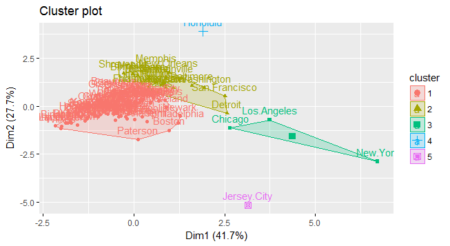
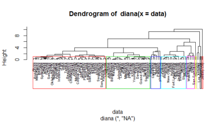
You can also visualize the clusters inside the dendogram itself by putting borders as shown next
pltree(hc4, hang=-1, cex = 0.6)


rect.hclust(hc4, k = 9, border = 2:10)

dendextend

You can do a lot of other manipulation on dendrograms with the dendextend package such as – changing the color of labels, changing the size of text of labels, changing type of line of branches, its colors, etc. You can also change the label text as well as sort it. You can see the many options in the online vignette of the package.

Another important function that the dendextend package offers is tanglegram. It is used to compare two dendrogram (with the same set of labels), one facing the other, and having their labels connected by lines.

As an example, let’s compare the single and complete linkage methods for agnes function.

library(dendextend)

hc_single <- agnes(data, method = "single")
hc_complete <- agnes(data, method = "complete")

# converting to dendogram objects as dendextend works with dendogram objects 
hc_single <- as.dendrogram(hc_single)
hc_complete <- as.dendrogram(hc_complete)

tanglegram(hc_single,hc_complete)

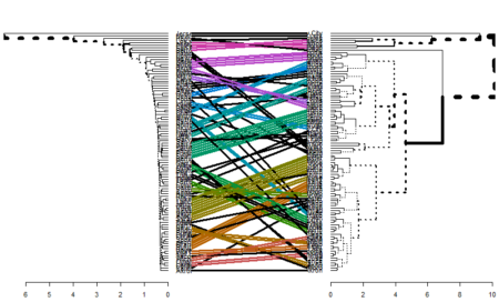
This is useful in comparing two methods. As seen in the figure, one can relate to the methodology used for building the clusters by looking at this comparison. You can find more functionalities of the dendextend package here.

End Notes

Hope now you have a better understanding of clustering algorithms than what you started with. We discussed about Divisive and Agglomerative clustering techniques and four linkage methods namely, Single, Complete, Average and Ward’s method. Next, we implemented the discussed techniques in R using a numeric dataset. Note that we didn’t have any categorical variable in the dataset we used. You need to treat the categorical variables in order to incorporate them into a clustering algorithm. Lastly, we discussed a couple of plots to visualise the clusters/groups formed. Note here that we have assumed value of ‘k’ (number of clusters) is known. However, this is not always the case. There are a number of heuristics and rules-of-thumb for picking number of clusters. A given heuristic will work better on some datasets than others. It’s best to take advantage of domain knowledge to help set the number of clusters, if that’s possible. Otherwise, try a variety of heuristics, and perhaps a few different values of k.

Consolidated code

install.packages('cluster')
install.packages('purrr')
install.packages('factoextra')

library(cluster)
library(purrr)
library(factoextra)
data <- car::Freedman
data <- na.omit(data)
data <- scale(data)

d <- dist(data, method = "euclidean")
hc1 <- hclust(d, method = "complete" )

plot(hc1, cex = 0.6, hang = -1)

hc2 <- agnes(data, method = "complete")
hc2$ac

m <- c( "average", "single", "complete", "ward")
names(m) <- c( "average", "single", "complete", "ward")

ac <- function(x) {
  agnes(data, method = x)$ac
}

map_dbl(m, ac)  

hc3 <- agnes(data, method = "ward")
pltree(hc3, cex = 0.6, hang = -1, main = "Dendrogram of agnes")

hc4 <- diana(data)
hc4$dc

pltree(hc4, cex = 0.6, hang = -1, main = "Dendrogram of diana")

clust <- cutree(hc4, k = 5)
fviz_cluster(list(data = data, cluster = clust))

pltree(hc4, hang=-1, cex = 0.6)
rect.hclust(hc4, k = 9, border = 2:10)

library(dendextend)

hc_single <- agnes(data, method = "single")
hc_complete <- agnes(data, method = "complete")

# converting to dendogram objects as dendextend works with dendogram objects 
hc_single <- as.dendrogram(hc_single)
hc_complete <- as.dendrogram(hc_complete)

tanglegram(hc_single,hc_complete)

Author Bio:

This article was contributed by Perceptive Analytics. Amanpreet Singh, Chaitanya Sagar, Jyothirmayee Thondamallu and Saneesh Veetil contributed to this article.

Perceptive Analytics provides data analytics, business intelligence and reporting services to e-commerce, retail and pharmaceutical industries. Our client roster includes Fortune 500 and NYSE listed companies in the USA and India.