(This is NOT financial advice, and the content is only for educational purposes)
Introduction to CPPI strategy
The Constant Proportion Portfolio Insurance (CPPI) strategy is a risk management technique that dynamically adjusts the allocation of an investment portfolio between risky and safe assets. The goal of the strategy is to ensure that a minimum level of wealth is maintained, while also participating in potential gains from risky assets. Introduced convex option-like payoffs, but without using options.
With a simple case of two assets, it is ou’re going
Getting Started
To implement the CPPI strategy, we will need the following R packages:
quantmod: to download the Bitcoin historical data.ggplot2: for graphics.
To implement the CPPI strategy we will use Bitcoin as the risky asset. We will download the monthly historical data from Yahoo Finance using the getSymbols function from the quantmod package. We will then calculate the monthly returns using the Return.calculate function. We will assume a risk-free rate of 2% (per annum).
CPPI Strategy
To implement the strategy we need the following inputs:
S: numeric: returns path of risky asset.multiplier: numericfloor: numeric: a percentage, should be smaller than 1.r: numeric: interest rate (per time period tau).tau: numeric: time periods.
Implementing the CPPI strategy involves rebalancing frequently to guarantee that the investments will never breach the floor. The absence of transaction costs using Bitcoin data allows a costless frequent rebalance. However, when trading other assets, such as for example traded ETFs, transaction costs should be taken into account.
In the code below we will firstly show an implementation of the CCPI strategy with a static floor. We will them show an alternative that reset the floor in each time-period. We will backtest the CPPI strategy against a risky investment of 100% into Bitcoin as well as a buy-and-hold strategy with 60% invested in the risky asset (Bitcoin) and 40% invested in the safe asset.
library(ggplot2)
library(quantmod)

getSymbols("BTC-USD", from = "2020-01-06", to = Sys.Date(), auto.assign = TRUE)
bitcoin <- `BTC-USD`

# Calculate monthly returns of the Bitcoin series
btc_monthly <- to.monthly(bitcoin)[, 6]
btc_monthly_returns <- monthlyReturn(btc_monthly)
 r <– 0.02
risk_free_rate <- rep(r/12, length(btc_monthly_returns))

floor <- 0.8
multiplier <- 3 # so the investment is (1-0.8)*3 of the initial value, which is equivalent to a starting portfolio with 60/40 strategy
start_value <- 1000 # Initial investment
date <- index(btc_monthly_returns)
n_steps <- length(date)
account_value <- cushion <- risky_weight <- safe_weight <- risky_allocation <- safe_allocation <- numeric(n_steps)
account_value[1] <- start_value
floor_value <- floor*account_value
cushion[1] <- (account_value[1]-floor_value[1])/account_value[1]
risky_weight[1] <- multiplier * cushion[1]
safe_weight[1] <- 1-risky_weight[1]

risky_allocation[1] <- account_value[1] * risky_weight[1]
safe_allocation[1] <- account_value[1] * safe_weight[1]

risky_return <- cumprod(1+btc_monthly_returns)

# Static floor: horizontal line
for (s in 2:n_steps) {
  account_value[s] = risky_allocation[s-1]*(1+btc_monthly_returns[s]) + safe_allocation[s-1]*(1+risk_free_rate[s-1])
  floor_value[s] <- account_value[1] * floor
  cushion[s] <- (account_value[s]-floor_value[s])/account_value[s]
  risky_weight[s] <- multiplier*cushion[s]
  risky_weight[s] <- min(risky_weight[s], 1)
  risky_weight[s] <- max(0, risky_weight[s])
  safe_weight[s] <- 1-risky_weight[s]
  risky_allocation[s] <- account_value[s] * risky_weight[s]
  safe_allocation[s] <- account_value[s] * safe_weight[s]
}
buy_and_hold <- cumprod(1+(0.6*btc_monthly_returns + 0.4*risk_free_rate))

z_static <- cbind(account_value/1000, risky_return, buy_and_hold, floor_value/1000)

# Rename the columns
colnames(z_static) <- c("CPPI", "Bitcoin", "Mixed", "Floor_Value")

ggplot(z_static, aes(x = index(z_static))) +
  geom_line(aes(y = CPPI, color = "CPPI")) +
  geom_line(aes(y = Bitcoin, color = "Bitcoin")) +
  geom_line(aes(y = Mixed, color = "60-40")) +
  geom_line(aes(y = Floor_Value, color = "Floor Value")) +
  labs(title = "CPPI Strategy with Static Floor",
       x = "Time",
       y = "Cumulated Return",
       color = "Strategy") +
  theme_bw()

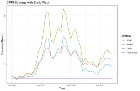
The plot shows that the CPPI strategy allows not to breach the floor at the beginning of the series. Then, the more it deviates from the floor the greater is the allocation in the risky asset up to 100% exceeding the 60/40 strategy to end up below the other strategies at the end of the backtesting period. A floor that does not change over time is not very helpful as we end up with a similar strategy to the 60/40 buy and hold where the downside protection seems ineffective. The next algorithm is build to allow for a floor that resets automatically with new highs of the risky allocation.
# Dynamic Floor: step wise update of the floor
peak <- dynamic_floor <- numeric(n_steps)

peak[1] <- start_value
dynamic_floor <- floor*account_value

for (s in 2:n_steps) {
  account_value[s] = risky_allocation[s-1]*(1+btc_monthly_returns[s]) + safe_allocation[s-1]*(1+risk_free_rate[s-1])

  peak[s] <- max(start_value, cummax(account_value[1:s]))
  dynamic_floor[s] <- floor*peak[s]

  cushion[s] <- (account_value[s]-dynamic_floor[s])/account_value[s]
  risky_weight[s] <- multiplier*cushion[s]
  risky_weight[s] <- min(risky_weight[s], 1)
  risky_weight[s] <- max(0, risky_weight[s])
  safe_weight[s] <- 1-risky_weight[s]
  risky_allocation[s] <- account_value[s] * risky_weight[s]
  safe_allocation[s] <- account_value[s] * safe_weight[s]
}

z_dynamic <- cbind(account_value/start_value, risky_return, buy_and_hold, dynamic_floor/start_value)

# Rename the columns
colnames(z_dynamic) <- c("CPPI", "Bitcoin", "Mixed", "Floor_Value")

ggplot(z_dynamic, aes(x = index(z_dynamic))) +
  geom_line(aes(y = CPPI, color = "CPPI")) +
  geom_line(aes(y = Bitcoin, color = "Bitcoin")) +
  geom_line(aes(y = Mixed, color = "60-40")) +
  geom_line(aes(y = Floor_Value, color = "Dynamic Floor")) +
  labs(title = "CPPI Strategy with Dynamic Floor",
       x = "Time",
       y = "Cumulated Return",
       color = "Strategy") +
  theme_bw()
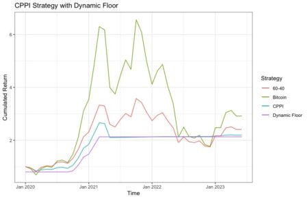
 The new algorithm works similarly to a dynamic call option that resets a new floor for each new high. The reallocation in the safe asset allows to completely offsets losses after Jan 2021, while fully taking advantage of the upside up until then. How do our strategies compare with each other? To answer this question we compare Annualised returns, volatility and Sharpe ratios for both CPPI strategies as well as 60/40 strategy and risky portfolio invested 100% in Bitcoins.
# Annualized returns
 bh_aret_st <- as.numeric((buy_and_hold[length(buy_and_hold)])^(12/n_steps)-1) # Buy-and-Hold strategy
bitcoin_aret_st <- as.numeric((risky_return[length(risky_return)])^(12/n_steps)-1) # Risky returns
cppi_aret_st <- (account_value[length(account_value)]/start_value)^(12/n_steps)-1 # Static CPPI
cppi_aret_dyn <- (account_value[length(account_value)]/start_value)^(12/n_steps)-1 # Dynamic CPPI

# Volatility and annualized volatility
bh_vol_st <- sd(0.6*btc_monthly_returns + 0.4*risk_free_rate)
bitcoin_vol_st <- sd(btc_monthly_returns)
cppi_vol_st <- sd(risky_weight*btc_monthly_returns + safe_weight*risk_free_rate)
cppi_vol_dyn <- sd(risky_weight*btc_monthly_returns + safe_weight*risk_free_rate)

bh_avol_st <- bh_vol_st*sqrt(12)
bitcoin_avol_st <- bitcoin_vol_st*sqrt(12)
cppi_avol_st <- cppi_vol_st*sqrt(12)
cppi_avol_dyn <- cppi_vol_dyn*sqrt(12)

# Sharpe Ratios
bh_sr_st <- (bh_aret_st-0.02)/bh_avol_st
bitcoin_sr_st <- (bitcoin_aret_st-0.02)/bitcoin_avol_st
cppi_sr_st <- (cppi_aret_st-0.02)/cppi_avol_st
cppi_sr_dyn <- (cppi_aret_dyn-0.02)/cppi_avol_dyn

summary <- c(bitcoin_aret_st, bitcoin_avol_st, bitcoin_sr_st, bh_aret_st, bh_avol_st, bh_sr_st, cppi_aret_st, cppi_avol_st, cppi_sr_st, cppi_aret_dyn, cppi_avol_dyn, cppi_sr_dyn)
summary <- matrix(summary, nrow=3,ncol=4,byrow=FALSE, dimnames=list(c("Average return","Annualised Vol","Sharpe Ratio"), c("Bitcoin", "Buy-and-hold", "CPPI Static Floor", "CPPI Dynamic Floor")))
round(summary, 2)

                 Bitcoin   Buy-and-hold CPPI Static  CPPI Dynamic
Average return   0.34      0.27         0.18         0.25
Annualised Vol   0.73      0.44         0.68         0.27
Sharpe Ratio     0.43      0.58         0.23         0.86
The fully risk-on portfolio with 100% invested in Bitcoin has the highest annualised return (34%), but also the highest volatility (73%). While there is not much benefit of implementing the static CPPI strategy (lowest Sharpe ratio at 0.23) vs for example a simple buy-and-hold, the dynamic CPPI shows much superior performances. The Sharpe ratio for the dynamic CPPI strategy is significantly higher than all other strategies, mainly due to a lower volatility without sacrificing much returns.