This is my very first post… many researchers / students / practitioners from all over the world write to me regularly about my R package SystemicR. I’m glad to contribute to the community but questions about data management and plotting often come up. I guess that the package notice could be improved. As I receive more and more emails (which I always answer), I have to go a step further. In order to help the community in the most efficient way, I am launching a blog ! The purpose is to introduce my package proposing a tutorial. I hope you’ll find what you were looking for !
Tutorial : load, estimate and plot
First of all, you have to install and load the package SystemicR (available on CRAN so that’s the easy part) :
# Install and load SystemicR

install.packages("SystemicR")

library(SystemicR)
See ? By the way I use RStudio / R 3.6.3, please let me know in comments if you have problems with more recent versions.
Then, we have to deal with data input : (i) the data I used in my research paper entitled “Systemic Risk: a Network Approach”, or (ii) your own data. Let’s begin with my data (included in the package) :
# Data management

data("data_stock_returns")

head(data_stock_returns)

data("data_state_variables")

head(data_state_variables)
That’s it. Nothing too difficult. But things can be a bit more complicated if you choose to import your own data. First of all, you have to be very careful about the input file: please import a .txt or .csv file. This will avoid 90% of the issues you face and write to me about. Then, you have to be aware of the format of the variables that the functions can take as input. The first column is named “Date” but the variable is not a date. I used a character format when I created this dataframe. If you want to import your own data, please use the “dd/mm/yyyy” format. Furthermore, my advice would be to import the data from a .txt or .csv file, using the command :
# Import data

df_my_data <- read.table(file = "My_CSV_File", sep = ";")

df_my_data <- read.csv(file = "My_CSV_File", sep = ";")
And please be careful about
sep =…Once data management is done, the remaining part of the code is straightforward. The package SystemicR is a toolbox that provides R users with useful functions to estimate and plot systemic risk measures.
Let’s begin with
f_CoVaR_Delta_CoVaR_i_q(). This function computes the CoVaR and the ΔCoVaR of a given financial institution i for a given quantile q. I developed this function following each step of Adrian and Brunnermeier (2016)’s research article :# Compute CoVaR_i_q and Delta_CoVaR_i_q
f_CoVaR_Delta_CoVaR_i_q(data_stock_returns) Then, having estimated this static measure, let’s move on to the dynamic using
f_CoVaR_Delta_CoVaR_i_q_t().Still, I developed this function following each step of Adrian and Brunnermeier (2016)’s research article :# Compute CoVaR_i_q_t , Delta_CoVaR_i_q_t and Delta_CoVaR_t
l_result <- f_CoVaR_Delta_CoVaR_i_q_t(data_stock_returns, data_state_variables) Of course, other systemic risk measures can be estimated. Following Billio et al. (2012), the function
f_correlation_network_measures() estimates degree, closeness centrality, eigenvector centrality. This function also estimates SR and volatility as in Hasse (2020):# Compute topological risk measures from correlation-based financial networks
l_result <- f_correlation_network_measures(data_stock_returns)
Last but not least, we shall now plot the evolution of one of the systemic risk measure using the function
f_plot() :# Plot Delta_CoVaR_t and SR_t
f_plot(l_result$Delta_CoVaR_t)
f_plot(l_result$SR) And that’s it! Before the end of the year, I will do my best to propose a new version of this package, including updated data and other systemic risk measure. Any suggestions are welcome and you can contact me if needed. Last, please do not hesitate to share your thoughts or questions above !
References
Adrian, Tobias, and Markus K. Brunnermeier. “CoVaR”. American Economic Review 106.7 (2016): , 106, 7, 1705-1741.
Billio, M., Getmansky, M., Lo, A. W., & Pelizzon, L. (2012). Econometric measures of connectedness and systemic risk in the finance and insurance sectors. Journal of Financial Economics, 104(3), 535-559.
Hasse, Jean-Baptiste. “Systemic Risk: a Network Approach”. AMSE Working Paper (2020)
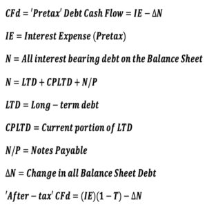
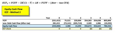
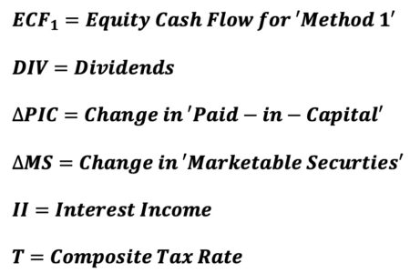
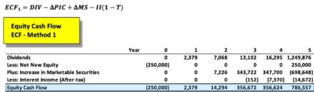
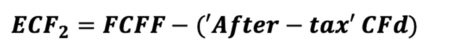 The equation appears innocent enough, though there are many underlying terms that require definition for understanding of the calculation. In words, ‘ECF – Method 2’ equals free cash Flow (FCFF) minus after-tax Debt Cash Flow (CFd).